This is the multi-page printable view of this section. Click here to print.
Tutorials
- 1: Getting Tensil to run ResNet at 300 frames per second on ZCU104
- 2: Building speech controlled robot with Tensil and Arty A7 - Part II
- 3: Building speech controlled robot with Tensil and Arty A7 - Part I
- 4: Learn how to combine Tensil and TF-Lite to run YOLO on Ultra96
- 5: Learn Tensil with ResNet and PYNQ Z1
- 6: Learn Tensil with ResNet and Ultra96
1 - Getting Tensil to run ResNet at 300 frames per second on ZCU104
Originally posted here.
Introduction
Sometimes the application requires pushing the performance to its limits. In this tutorial we will show how to optimize Tensil running ResNet20 trained on CIFAR for maximum performance. To do this, we will use the powerful ZCU104 board and implement an embedded application to remove the overhead of running Linux OS and PYNQ. Importantly, we still won’t quantize the model and use Tensil with 16-bit fixed point data type. We will demonstrate that running the CIFAR test data set shows very little accuracy drop when rounding down from the original 32-bit floating point.
We will be using Vivado 2021.1, which you can download and use for free for educational projects. Make sure to install Vitis, which will include Vivado and Vitis. We will use Vitis for building the embedded application.
Tensil tools are packaged in the form of Docker container, so you’ll need to have Docker installed and then pull Tensil Docker image by running the following command.
docker pull tensilai/tensil
Next, use docker run command to launch Tensil container.
docker run \
    -u $(id -u ${USER}):$(id -g ${USER}) \
    -v $(pwd):/work \
    -w /work \
    -it tensilai/tensil \
    bash
You will also need to clone the tutorial GitHub repository. It contains necessary source files as well as all of the intermediate artifacts in case you would like to skip running Tensil tools or Vivado.
Baseline solution
We start with the baseline solution, in which we will create a working Tensil application with default design choices. Once we have a stable working solution we will look at opportunities to improve its performance.
Tensil RTL and Vivado implementation
Let’s start with generating Tensil RTL. Run the following command to generate Verilog artifacts.
tensil rtl -a /demo/arch/zcu104.tarch -d 128 -s true -t vivado/baseline
You can skip running the Tensil RTL tool and grab the baseline Verilog artifacts here.
Note that we need to specify the data width for AXI interfaces to be 128 bits, so that they fit directly with AXI ports on the ZYNQ UltraScale+ device at the heart of the ZCU104 board.
Next, create the new Vivado RTL project, select the ZCU104 board and import the three Verilog files produced by the Tensil RTL command.
We provide scripted block design, so that you won’t need to connect blocks manually. You can use Tools -> Run Tcl Script to run it. Once you have the design ready, right-click on tensil_zcu104 in the Design Sources pane and select Create HDL Wrapper. Let Vivado manage the wrapper. Once the wrapper is ready, right-click on tensil_zcu104_wrapper in the same Design Sources pane and select Set as Top.
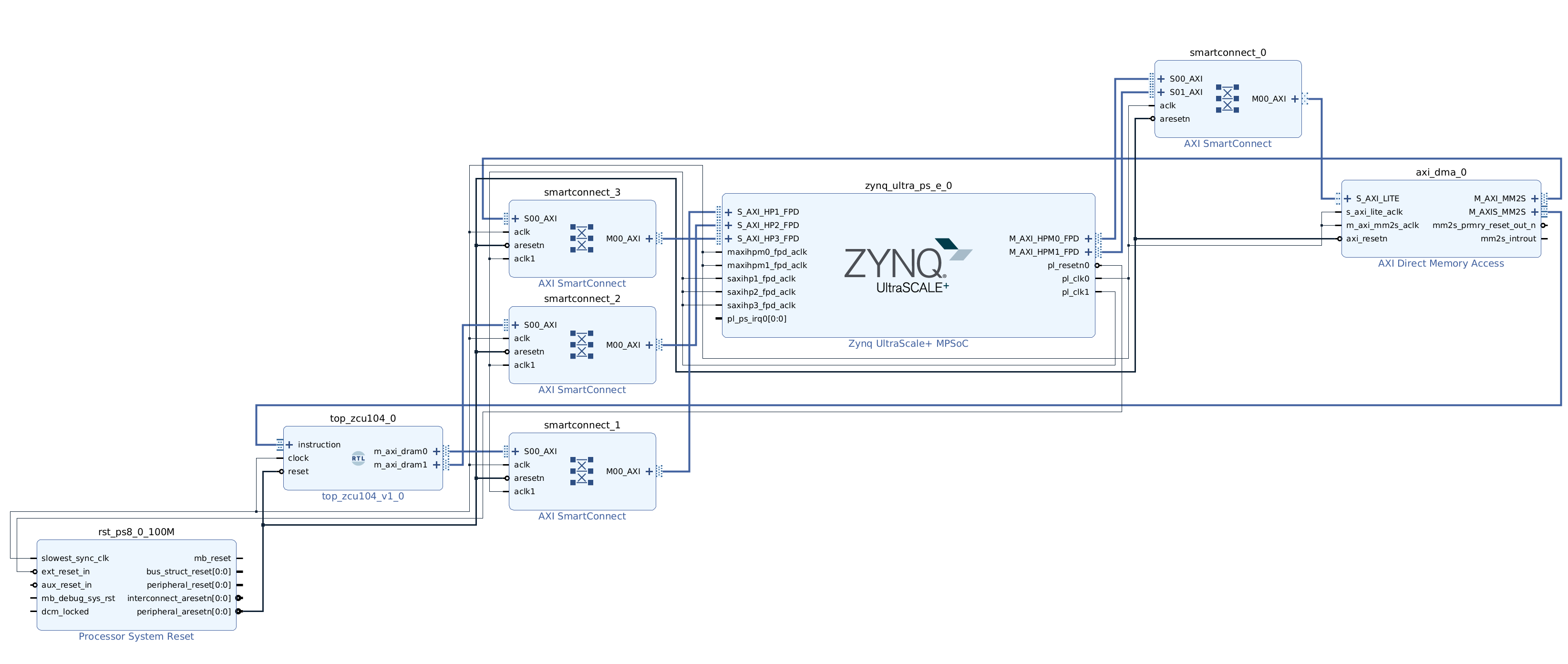
Following is how the baseline block design looks like. Note the direct connections between Tensil block AXI masters and ZYNQ AXI slaves. The instruction AXI stream port is connected via AXI DMA block.
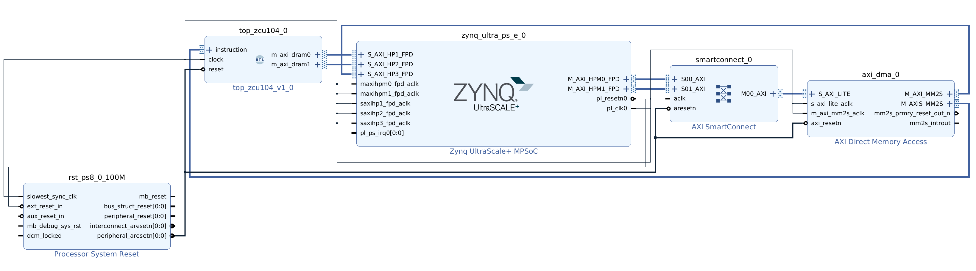
Next, click on Generate Bitstream in the Flow Navigator pane. Once bitstream is ready click on File -> Export -> Export Hardware. Make sure that Include bitstream choice is selected. Now you have the XSA file containing everything necessary for Vitis to create the embedded application project.
You can skip the Vivado implementation and grab the baseline XSA file here.
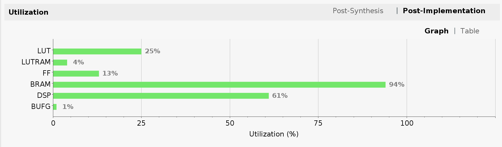
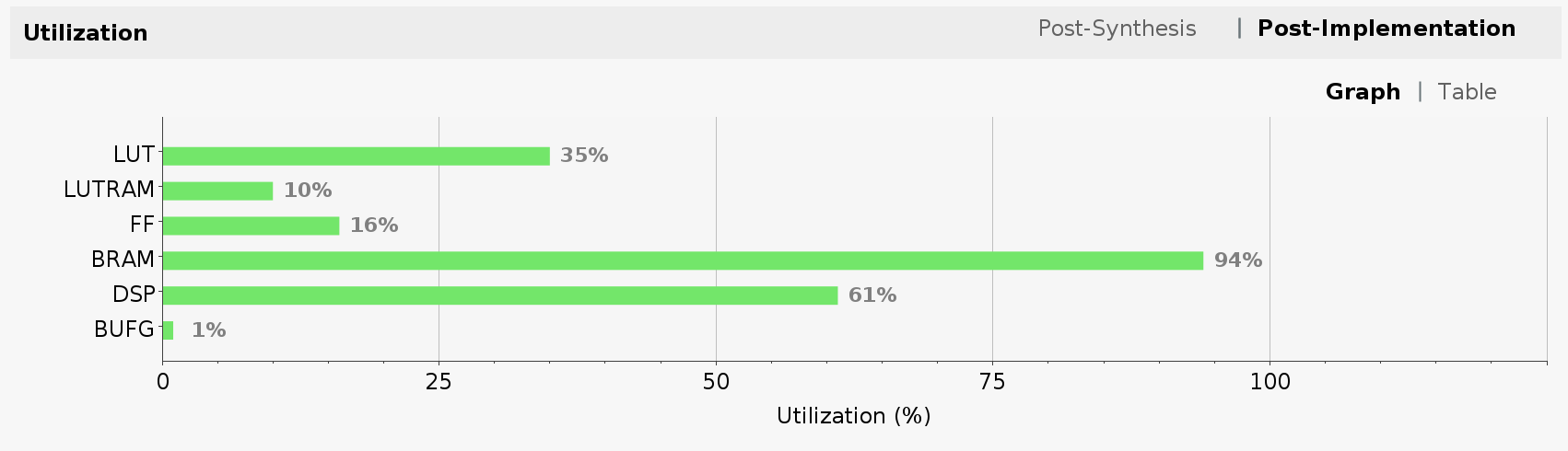
Another important result of running Vivado implementation is FPGA utilization. It is shown as one of the panes in the project summary once implementation is completed. The utilization is a direct function of our choice of Tensil architecture.
{
    "data_type": "FP16BP8",
    "array_size": 32,
    "dram0_depth": 2097152,
    "dram1_depth": 2097152,
    "local_depth": 16384,
    "accumulator_depth": 4096,
    "simd_registers_depth": 1,
    "stride0_depth": 8,
    "stride1_depth": 8,
    "number_of_threads": 1,
    "thread_queue_depth": 8
}
Specifying 32 by 32 systolic array size contributed to the high utilization of multiply-accumulate units (DSP). Note how we pushed Block RAM (BRAM) utilization almost to its limit by specifying 16 KV local memory and 4 KV accumulators (KV = 1024 vectors = 1024 * 32 * 16 bits).
ResNet compiled for Tensil
The ZCU104 board supports an SD card interface. This allows us to use Tensil embedded driver file system functionality to read the ResNet model and a set of images to test it with. The set we will be using is the test set for the original CIFAR-10. The ResNet model is trained with the separate training and validation sets from the CIFAR-10. The test set is what the model hasn’t seen in training and therefore gives an objective estimate of its accuracy. The CIFAR-10 provides the test set of 10,000 images in several formats. We will use the binary format that is more suitable for the embedded application.
Let’s start with compiling the ResNet ONNX file to Tensil model artifacts. The following command will produce *.tmodel, *.tdata and *.tprog files under the sdcard/baseline/ directory. The *.tmodel file is a JSON-formatted description of the Tensil model, which references *.tdata (model weights) and *.tprog (model program for the Tensil processor.)
tensil compile \
    -a /demo/arch/zcu104.tarch \
    -m /demo/models/resnet20v2_cifar.onnx \
    -o "Identity:0" \
    -s true \
    -t sdcard/baseline/
Once compiled, copy the content of the sdcard directory, which should also include the CIFAR-10 test data set (test_batch.bin) to the FAT-formatted SD card. Insert the card into the ZCU104 SD card slot.
You can skip the model compilation step and use the sdcard directory in our GitHub repository.
Tensil for Vitis embedded applications
Launch Vitis IDE and create a new workspace for our project. Once greeted by the welcome screen click on Create Application Project. On the subsequent screen select Create a new platform from hardware (XSA) and select the XSA file produced in the previous section. Name the application project tensil_zcu104. Keep default choices in the next few screens. On the last screen select Empty Application (C).
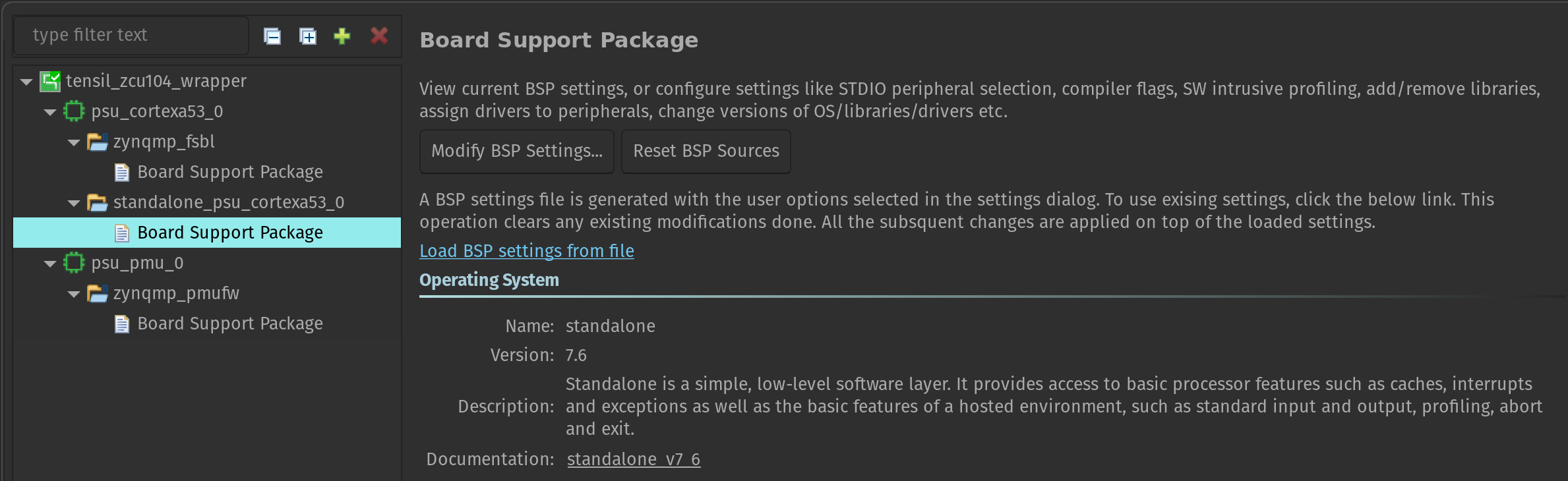
Now let’s make one important adjustment to the platform. Right-click on the tensil_zcu104 [Application] project in the Assistant pane and select Navigate to BSP settings. You will see a tree containing psu_cortex53_0 (the ARM cores we will be running on) with zynqmp_fsbl (first stage bootloader) and standalone_psu_cortex53_0 (our application) subnodes. Board Support Package under standalone should be selected.
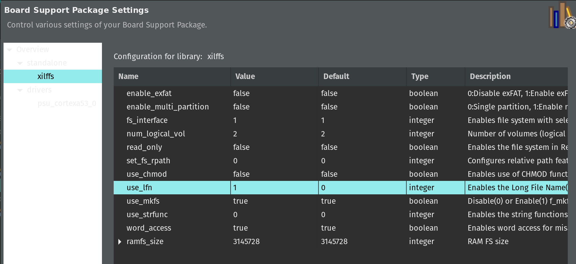
In the Board Support Package pane click on Modify BSP settings. In Overview click the checkbox for xilff. This will enable the FAT filesystem driver for the SD card slot supported by the ZCU104 board. Click on xilff that should have appeared under Overview in the left-side pane. Change use_lfn from 0 to 1. This will enable long file name support for the FAT filesystem driver.
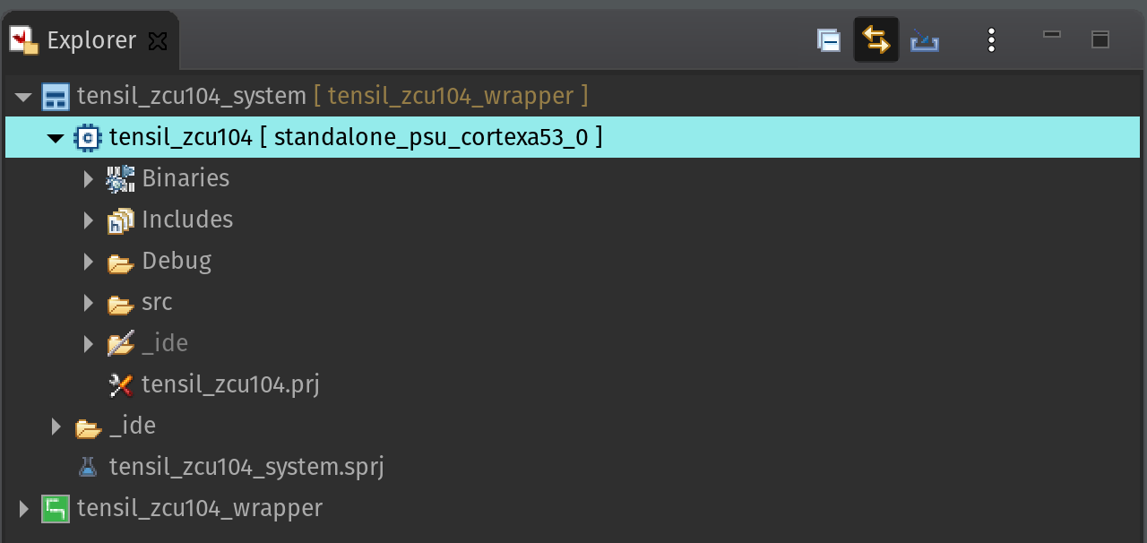
Before we copy all necessary source files, let’s adjust application C/C++ build settings to link our application with the standard math library. In the Explorer pane right-click the tensil_zcu104 application project. Select C/C++ Build Settings from the menu.
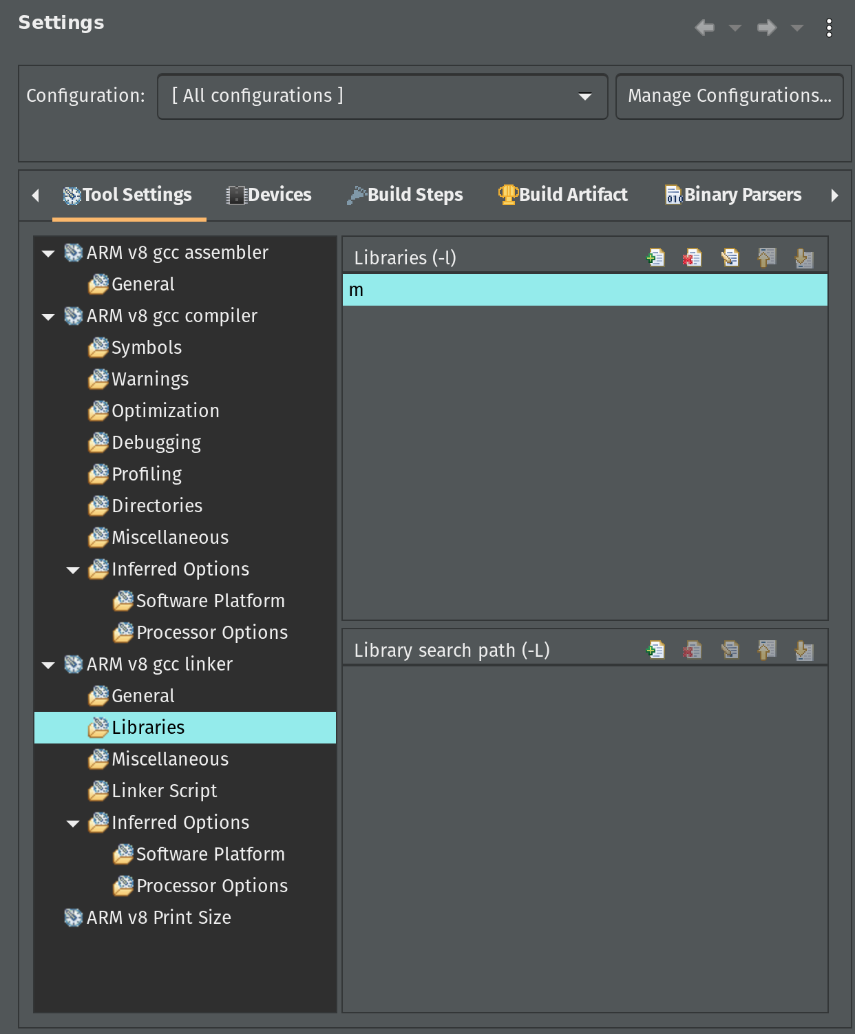
Click on Configuration dropdown and choose All configurations. Then, under ARM v8 gcc linker click on Libraries. In the Libraries pane click on the add button and enter m.
Now, let’s copy all necessary source files. For this you will need to clone the tutorial GitHub repository as well as the Tensil GitHub repository for the embedded driver sources. But first, let’s copy architecture parameters for the embedded driver from the output artifacts of Tensil RTL tool.
cp \
    <tutorial repository root>/vivado/baseline/architecture_params.h \
    <Vitis workspace root>/tensil_zcu104/src/
Next, copy the embedded driver.
cp -r \
    <Tensil repository root>/drivers/embedded/tensil \
    <Vitis workspace root>/tensil_zcu104/src/
Lastly, copy the ZCU104 embedded application. Note that platform.h copied in the previous step gets overwritten.
cp -r \
    <tutorial repository root>/vitis/* \
    <Vitis workspace root>/tensil_zcu104/src/
Finally, let’s build and run the application. First, make sure the ZCU104 board has boot DIP switches (SW6) all in ON position (towards the center of the board) to enable booting from JTAG. Then, right-click on the Debug entry under the tensil_zcu104 [Application] project in the Assistant pane and select Debug -> Launch Hardware.
Start the serial IO tool of your choice (like tio) and connect to /dev/ttyUSB1 at 115200 baud. It could be a different device depending on what else is plugged into your computer. Look for a device name starting with Future Technology Devices International.
tio -b 115200 /dev/ttyUSB1
With the SD card inserted and containing the CIFAR-10 test data set and the ResNet model compiled for Tensil you should see the inference printing every 100’s image and the corresponding prediction along with measured inferences (frames) per second.
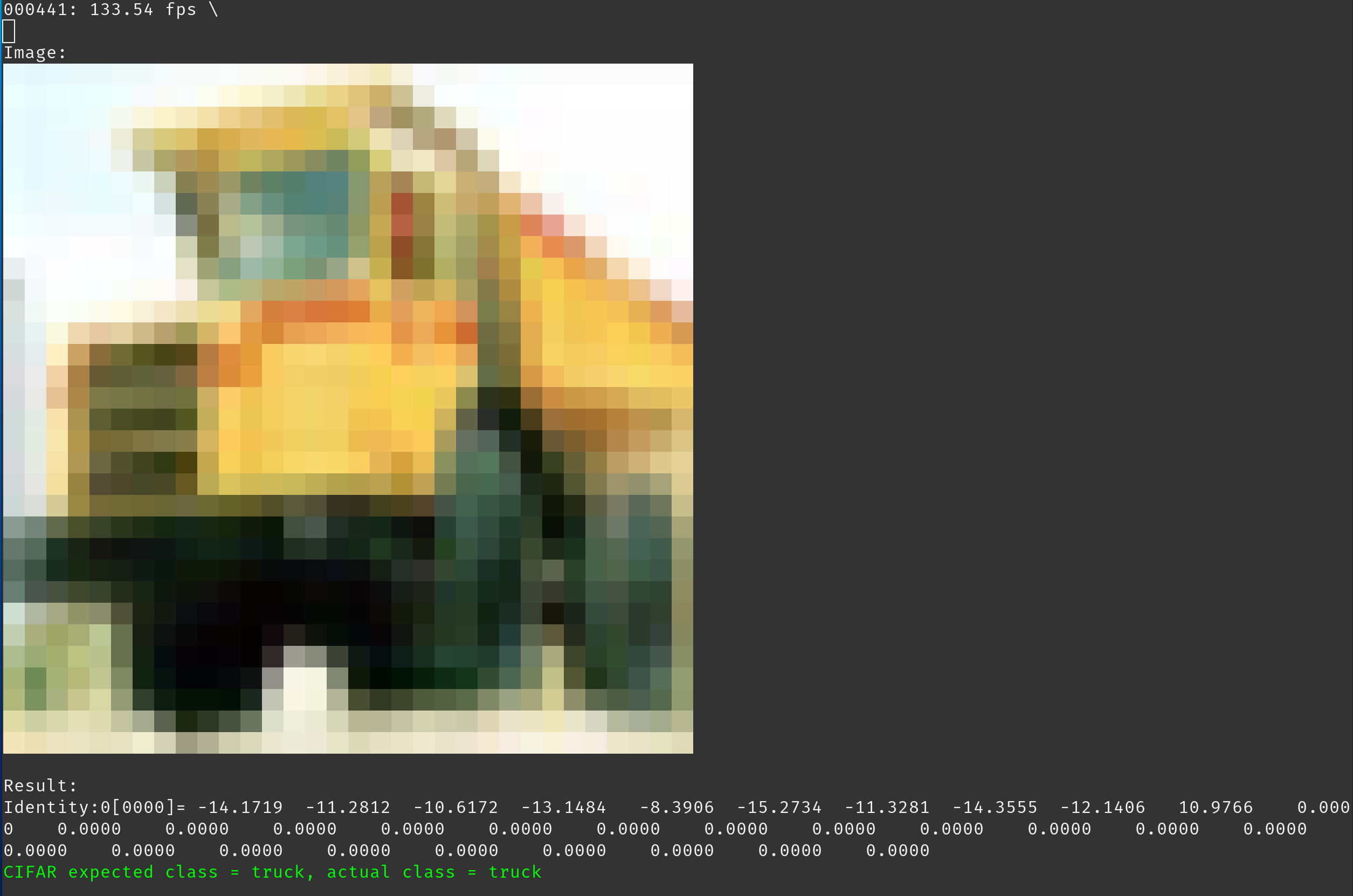
After running the inference on the entire test data set the program will print the final average frames per second and the accuracy of the inference. For the baseline solution we are getting an average of 133.54 frames per second with 90% accuracy. Note that the accuracy we are seeing when testing the same ResNet model with TensorFlow is 92%. The 2% drop is due to changing the data type from 32-bit floating point in TensorFlow to 16-bit fixed point in Tensil.
Dual clock solution
The first optimization is based on the following observation. The Tensil RTL block is clocked at 100MHz. (We could clock it higher, but for the purpose of this tutorial let’s assume this is our maximum clock.) The Tensil block DRAM0 and DRAM1 ports are connected to AXI interfaces on the ZYNQ block. The instruction port is indirectly connected to the AXI on the ZYNQ block via AXI DMA. ZYNQ UltraScal+ AXI ports support up to 333MHz and the maximum width of 128 bits. This gives us the opportunity to introduce a second clock domain for 333MHz while at the same time making the Tensil AXI ports wider.
The following diagram shows how this may work in a simpler 100MHz to 400MHz, 512- to 128-bit conversion. Each clock in the Tensil clock domain would pump one 512-bit word in or out. This would match 4 clocks in the ZYNQ clock domain with 512-bit word split to or composed from 4 128-bit words.

First let’s use the -d argument in Tensil RTL command to generate the RTL with 512-bit interfaces.
tensil rtl -a /demo/arch/zcu104.tarch -d 512 -s true -t vivado/dual_clock
The AXI SmartConnect block allows for both AXI width adjustment and separate clock domains. We change our block design by inserting these blocks in all three connections between Tensil RTL and the ZYNQ AXI ports. We suggest following the steps above to create a new Vivado project for the dual clock design. Again, we provide scripted block design, so that you won’t need to connect blocks manually. Following is how the dual clock block design looks like.
You can skip the Vivado implementation and grab the dual clock XSA file here.
Let’s take a look at FPGA utilization for dual clock design. Note that the utilization for LUT, LUTRAM and FF has increased due to added AXI SmartConnect blocks and wider Tensil intefaces. BRAM and DSP utilization stayed the same since we did not change the Tensil architecture.
Now, we suggest you also create a new Vitis workspace for the dual clock design and follow the steps above to get the inference running. The model remains unchanged since we did not change the Tensil architecture.
For the dual clock solution we are getting an average of 152.04 frames per second–a meaningful improvement over the baseline. This improvement is roughly proportional to the ratio of time spent in moving data to and from the FPGA to the time spent in internal data movement and computation.
Ultra RAM solution
The second optimization is based on the higher-end ZYNQ UltraScale+ devices support for another type of on-chip memory called Ultra RAM. By default, Vivado maps dual-port memory to Block RAM. In order for it to map to the Ultra RAM it needs hints in the Verilog code. To enable these hints we will use --use-xilinx-ultra-ram option of the Tensil RTL tool. The amount of Ultra RAM available on ZCU104 allows us to add around 48 KV memory in addition to 20 KV available through Block RAM.
We start by creating a new Tensil architecture for ZCU104 in which we allocate all of the Block RAM (20 KV) to accumulators and all of the Ultra RAM (48 KV) to local memory.
{
    "data_type": "FP16BP8",
    "array_size": 32,
    "dram0_depth": 2097152,
    "dram1_depth": 2097152,
    "local_depth": 49152,
    "accumulator_depth": 20480,
    "simd_registers_depth": 1,
    "stride0_depth": 8,
    "stride1_depth": 8,
    "number_of_threads": 1,
    "thread_queue_depth": 8
}
Run the following command to generate Verilog artifacts.
tensil rtl \
    -a /demo/arch/zcu104_uram.tarch \
    -d 512 \
    --use-xilinx-ultra-ram true \
    -s true \
    -t vivado/ultra_ram
You can also skip running the Tensil RTL tool and grab the Ultra RAM Verilog artifacts here.
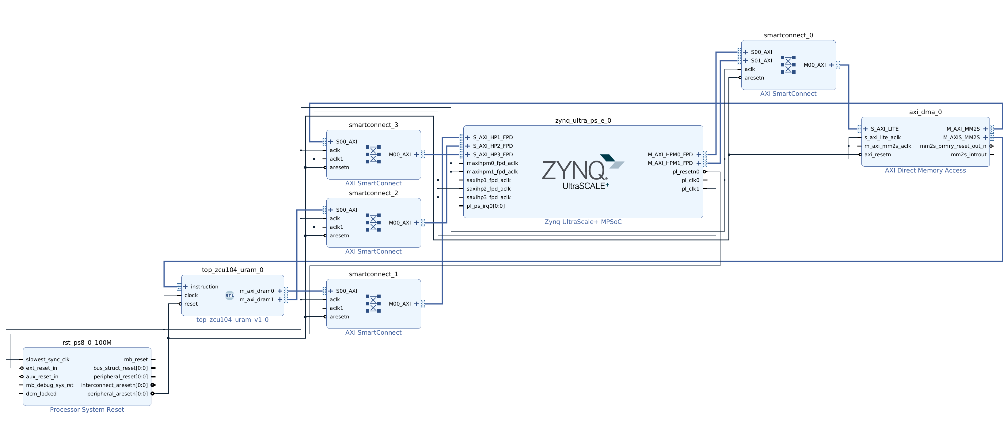
Follow the steps above to create a new Vivado project for Ultra RAM solution. We provide scripted block design, so that you won’t need to connect blocks manually. Following is how the Ultra RAM block design looks like. Note, that we based it on the dual clock design and the only difference is in the Tensil RTL block.
You can skip the Vivado implementation and grab the Ultra RAM XSA file here.
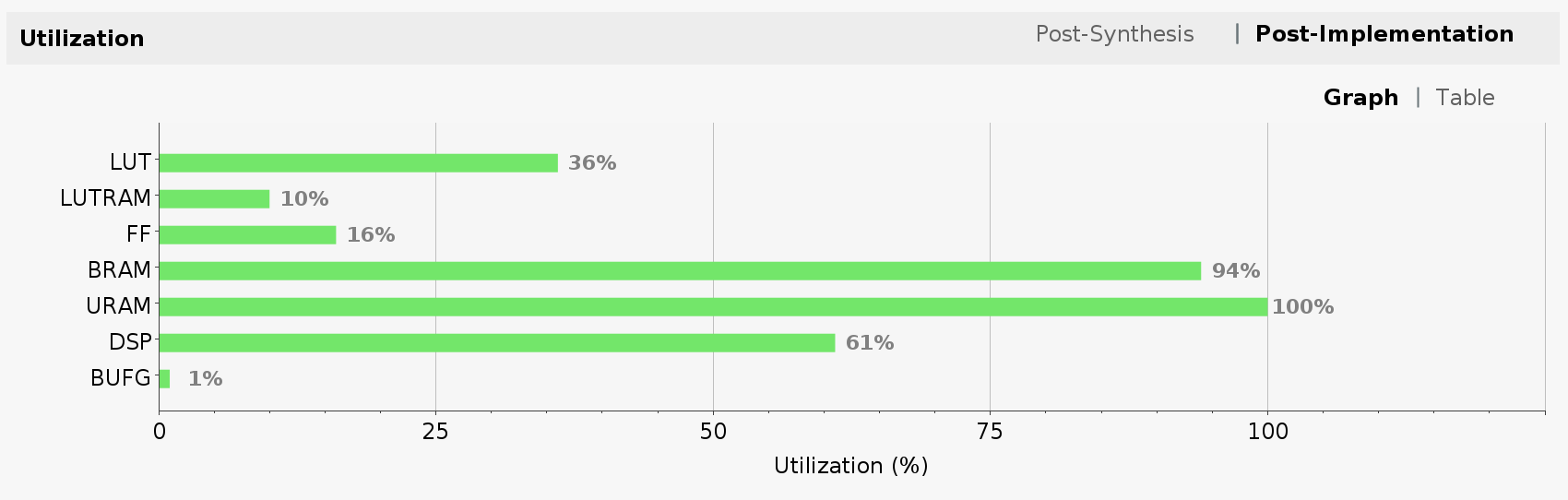
Now, let’s take a look at FPGA utilization for Ultra RAM design. Note that the utilization is mostly unchanged from the one of the dual clock design. The exception is the new line item for Ultra RAM (URAM), which we pushed to its full limit.
Because we changed the Tensil architecture the new model needs to be compiled and copied to the SD card.
tensil compile \
    -a /demo/arch/zcu104_uram.tarch \
    -m /demo/models/resnet20v2_cifar.onnx \
    -o "Identity:0" \
    -s true \
    -t sdcard/ultra_ram/
You can skip the model compilation step and use the sdcard directory in our GitHub repository.
We again, suggest you create a new Vitis workspace for the Ultra RAM design and follow the steps above to get the inference running. Make sure to uncomment the correct MODEL_FILE_PATH definition for the newly created *.tmodel file.
For the Ultra RAM solution we are getting an average of 170.16 frames per second, another meaningful improvement. This improvement is based purely on having larger on-chip memory. With a small on-chip memory the Tensil compiler is forced to partition ResNet convolution layers into multiple load-compute-save blocks. This, in turn, requires that the same input activations are loaded multiple times, assuming weights are loaded only once. This is called weight-stationary dataflow. In the future, we will add an option for input-stationary dataflow. With it, when partitioned, the input activations are loaded once and the same weights are loaded multiple times.
The following diagram shows such partitioned compilation. Layer N has 2 stages. In each stage a unique subset of weights is loaded. Then, each stage is further split into 2 partitions. Partition is defined by the largest amount of weights, input and output activations, and intermediate results that fit local memory and accumulators.

Having larger on-chip memory reduces this partitioning and, by extension, the need to load the same data multiple times. The following diagram shows how layer N now has 1 stage and 1 partition that fits larger local memory and accumulators, which allows weights and activations to be loaded only once.

Solutions with large local memory
The final optimization is based on the same hardware design and Tensil architecture we created to support the Ultra RAM. We will only change the Tensil compiler strategy.
As we mentioned previously, the Tensil compiler, by default, assumes that model is much larger in terms of its weights and activations than the local memory available on the FPGA. This is true for large models and for low-end FPGA devices. For small and medium sized models running on large FPGA devices there is a possibility that local memory is large enough to contain the weights plus input and output activations for each layer.
To see if this strategy is worth trying, we first look at the output of Tensil compiler for the ZCU104 architecture with the Ultra RAM.

The maximum number for stages and partitions being both 1 inform us that none of the layers were partitioned, or, in other words, each layer’s weights and activations did fit in the local memory. Another way to guide this decision is to use the --layers-summary true option with the Tensil compiler, which will report the summary per each layer with local and accumulator utilization.

Thus, the first strategy will be to try keeping activations in local memory between layers by specifying --strategy local-vars. The following diagram shows this strategy.

Run the following command and then copy the newly created model to the SD card.
tensil compile \
    -a /demo/arch/zcu104_uram.tarch \
    -m /demo/models/resnet20v2_cifar.onnx \
    -o "Identity:0" \
    -s true \
    --strategy local-vars \
    -t sdcard/ultra_ram_local_vars/
You can skip all of the model compilation steps in this section and use the sdcard directory in our GitHub repository.
This time, you can reuse the Vitis workspace for the Ultra RAM solution and simply uncomment the correct MODEL_FILE_PATH definition for each newly created *.tmodel file.
With the local-vars strategy we are getting an average of 214.66 frames per second.
Now that we have seen the improvement allowed by large on-chip memory, let’s see if any other load and save operations can be avoided. With local-vars strategy we load the input image and the weights and then save the output predictions. What if there would be enough on-chip memory to keep the weights loaded? There is a strategy for this!
With the local-consts strategy the inference expects all of the model weights to be preloaded to the local memory before the inference. This is the job for the driver. When the Tensil driver loads the model compiled with local-consts strategy it preloads its weights from *.tdata file into the local memory. The following diagram shows this strategy.

tensil compile \
    -a /demo/arch/zcu104_uram.tarch \
    -m /demo/models/resnet20v2_cifar.onnx \
    -o "Identity:0" \
    -s true \
    --strategy local-consts \
    -t sdcard/ultra_ram_local_consts/
With the local-consts strategy we are getting an average of 231.57 frames per second.
Finally, the local-vars-and-consts strategy combines local-vars and local-consts. With this strategy the inference will only load the input image and save the output predictions. The following diagram shows this strategy.

tensil compile \
    -a /demo/arch/zcu104_uram.tarch \
    -m /demo/models/resnet20v2_cifar.onnx \
    -o "Identity:0" \
    -s true \
    --strategy local-vars-and-consts \
    -t sdcard/ultra_ram_local_vars_and_consts/
With the local-vars-and-consts strategy we are getting an average of 293.58 frames per second.
Conclusion
In this tutorial we demonstrated how improving the Vivado hardware design, leveraging Xilinx Ultra RAM, and using the advanced compiler strategies can improve the performance of inference.
The following chart summarizes presented solutions and their frames per second performance.

2 - Building speech controlled robot with Tensil and Arty A7 - Part II
Originally posted here.
Introduction
This is part II of a two-part tutorial in which we will continue to learn how to build a speech controlled robot using Tensil open source machine learning (ML) acceleration framework, Digilent Arty A7-100T FPGA board, and Pololu Romi Chassis. In part I we focused on recognizing speech commands through a microphone. Part II will focus on translating commands into robot behavior and integrating with the Romi chassis.
System architecture
Let’s start by reviewing the system architecture we introduced in Part I. We introduced two high-level components: Sensor Pipeline and State Machine. Sensor Pipeline continuously receives the microphone signal as an input and outputs events representing one of the four commands. State Machine receives a command event and changes its state accordingly. This state represents what the robot is currently doing and is used to control the engine.

First, we will work on the State Machine and controlling the motors. After this we will wire it all together and assemble the robot on the chassis.

State Machine
The State Machine is responsible for managing the current state of the motors. It receives command events and depending on the command changes the motor’s state. For example, when it receives the “go!” command it turns both motors in the forward direction; when it receives the “right!” command it turns the right engine in the backward direction and the left engine in the forward direction.
The Sensor Pipeline produces events containing a command and its prediction probability. As we mentioned before the ML model is capable of predicting 12 classes of commands, from which our robot is using only 4. So, firstly, we filter events for known commands. Secondly, we use a per-command threshold to filter for sufficient probability. During testing these thresholds can be adjusted to find the best balance between false negatives and false positives for each command.
By experimenting with the Sensor Pipeline we can see that it may emit multiple events for the same spoken command. Usually, the series of these instances includes the same predicted command. This happens because the recognition happens on a sliding window where the sound pattern may be included in several consecutive windows. Occasionally, the series starts with a correctly recognized command and is then followed by an incorrect one. This happens when a truncated sound pattern in the last window gets mispredicted. To smooth out these effects we introduce a “debouncing” state. The debouncing state prevents changing the motor’s state for a fixed period of time after the most recent change.
Another effect observed with the Sensor Pipeline is that at the very beginning acquisition and spectrogram buffers are partially empty (filled with zeroes). This sometimes produces mispredictions right after the initialization. Therefore it will be useful to enter the debouncing state right after initialization.
Debouncing is implemented in the State Machine by introducing an equivalent of a wall clock. The clock is represented by the tick counter inside of the state structure. This counter is reset to its maximum at every motor’s state change and decremented at every iteration of the main loop. Once the clock is zero the State Machine transitions out of the debouncing state and starts accepting new commands.

You can look at the State Machine implementation in the speech robot source code.
Motor control
In order for the motors to turn, a difference in potential (voltage) must be applied to its M-(M1) and M+(M2) terminals. The strength and polarity of this voltage determines the speed and the direction of motion.
We use a HB3 PMOD to control this voltage with digital signals.
The polarity is controlled by a single digital wire. This value for left and right motors is produced by the Xilinx AXI GPIO component and is connected to MOTOR_DIR[1:0] pins on the PMODs. The State Machine is responsible for setting direction bits through the AXI GPIO register.
The strength of the voltage is regulated by the PWM waveform. This waveform has fixed frequency (2 KHz) and uses the ratio between high and low parts of the period (duty cycle) to specify the fraction of the maximum voltage applied to the motor. The following diagram from the HB3 reference manual shows how this works.
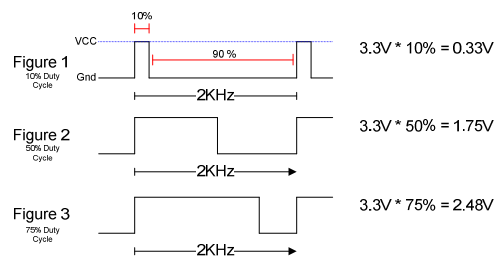
To generate the PWM waveform we use Xilinx AXI Timer. We used a dedicated timer instance for each motor to allow for independent speed control. The AXI Timer pwm output is connected to the MOTOR_EN pin on the PMODs. The State Machine is responsible for setting the total and high periods of the waveform through the AXI Timer driver from Xilinx.
You can look at the motor control implementation in the speech robot source code.
Assembling chassis
As the mechanical platform for the speech robot we selected Pololu Romi. This chassis is simple, easy to assemble and inexpensive. It also provides a built-in battery enclosure for 6 AA batteries as well as a nice power distribution board that outputs voltage sufficient for powering the motors and Arty A7 board. Pololu also provides an expansion plate for the chassis to conveniently place the Arty A7 board.
Following is a bill of material for all necessary components from Pololu.
Pololu includes an awesome video that details the process of assembling the chassis. Make sure you watch before starting to solder the power distribution board!
Before you place the power distribution board it’s time to warm your soldering iron. Solder two 8x1 headers to the VBAT, VRP, VSW terminals and the ground. You can use masking tape to keep the headers in place while soldering.

Next, place the power distribution board on the chassis so that battery terminals protrude through their corresponding holes. Use screws to secure it. Now, solder the terminals to the board.

Put the batteries in and press the power button. The blue LED should light up.
Next, solder a 6x1 headers to each of the motor encoder boards (Note! Use the same breakaway male header used with the power distribution board and not the one included with the encoder.) Then place an encoder board on each motor so that motor terminals protrude through the holes and solder them.

At last, insert motors into the chassis and wire them to HB3 PMODs (connect M- to M1 and M+ to M2). Wire the HB3 PMODs VM to one of the VSW terminals and GND to GND on the power distribution board. Plug the Arty A7 board and test everything together!
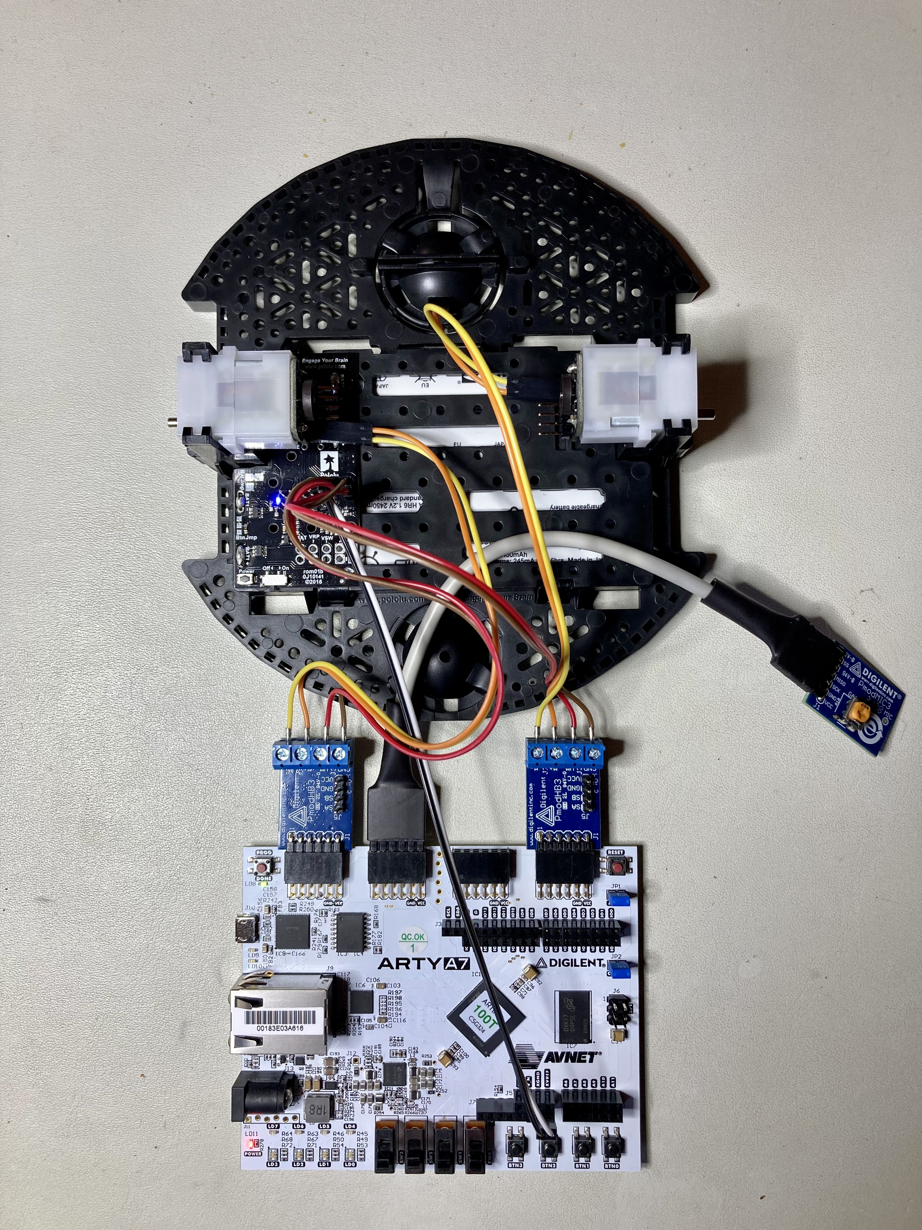
If everything works, continue with the final assembly. Connect two extension plates with 2 screws and mount it on the chassis using 4 standoffs. Mount wheels and the ball caster. Place Arty A7 board and HB3 PMODs on top of the surface formed by two extension plates. You can use two-side adhesive to keep them in place. We suggest using an 18-gauge wire to raise the MIC3 PMOD above the chassis to avoid the microphone being influenced by the noise of motors.
Conclusion
In part II of the tutorial we learned how to design the State Machine for the speech robot and how to interface with motor drivers. We then integrated all of the parts on the Pololu Romi chassis. Now that you have a functioning robot that obeys your commands, we invite you to extend it further and make use of the remaining 6 commands that our ML model can predict!
3 - Building speech controlled robot with Tensil and Arty A7 - Part I
Originally posted here.
Introduction
In this two-part tutorial we will learn how to build a speech controlled robot using Tensil open source machine learning (ML) acceleration framework and Digilent Arty A7-100T FPGA board. At the heart of this robot we will use the ML model for speech recognition. We will learn how Tensil framework enables ML inference to be tightly integrated with digital signal processing in a resource constrained environment of a mid-range Xilinx Artix-7 FPGA.
Part I will focus on recognizing speech commands through a microphone. Part II will focus on translating commands into robot behavior and integrating with the mechanical platform.
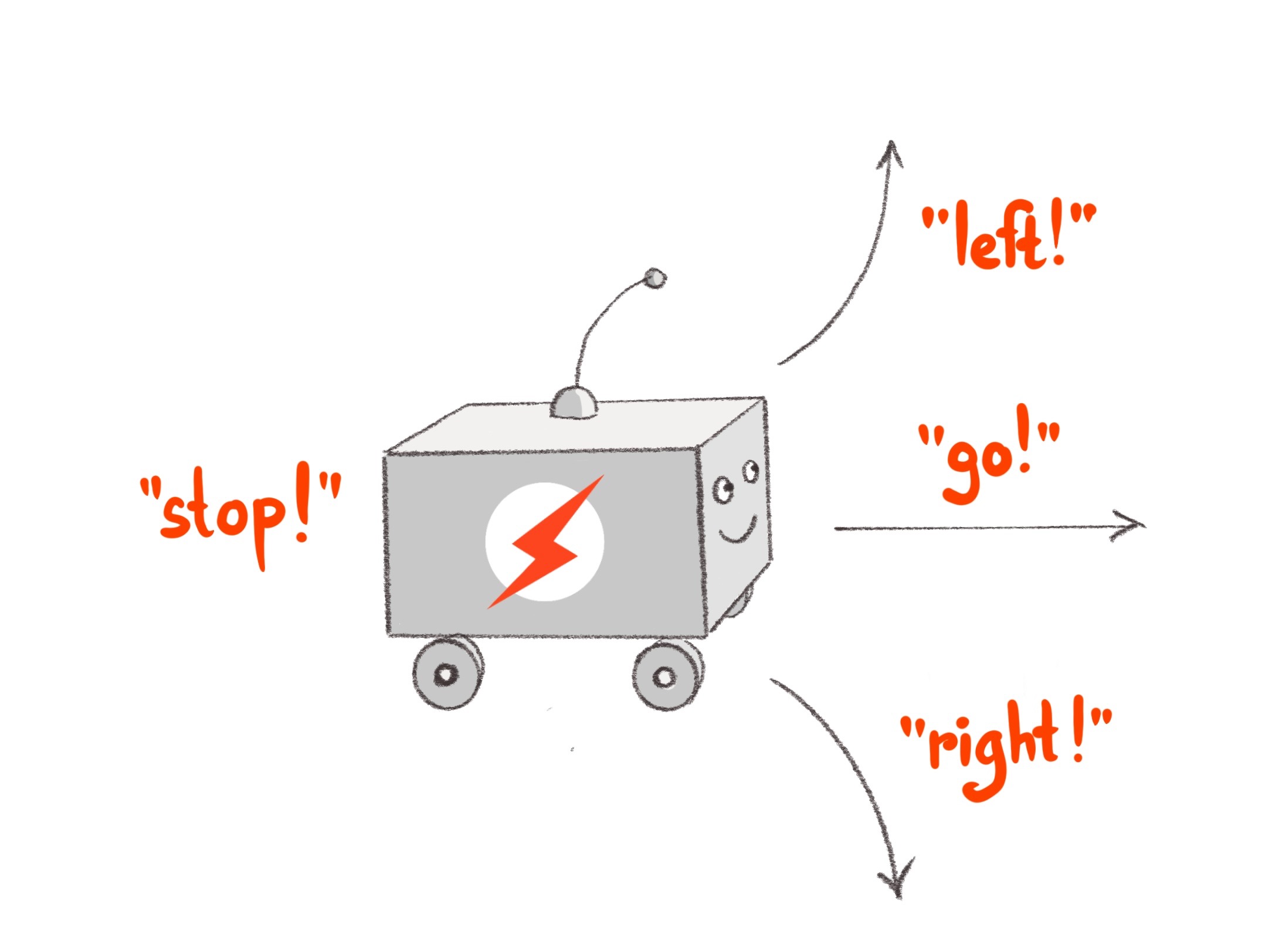
Let’s start by specifying what commands we want the robot to understand. To keep the mechanical platform simple (and inexpensive) we will build on a wheeled chassis with two engines. The robot will recognize directives to move forward in a straight line (go!), turn in-place clockwise (right!) and counterclockwise (left!), and turn the engines off (stop!).
System architecture
Now that we know what robot we want to build, let’s define its high-level system architecture. This architecture will revolve around the Arty board that will provide the “brains” for our robot. In order for the robot to “hear” we need a microphone. The Arty board provides native connectivity with the PMOD ecosystem and there is MIC3 PMOD from Digilent that combines a microphone with ADCS7476 analog-to-digital converter. And in order to control motors we need two HB3 PMOD drivers, also from Digilent, that will convert digital signals to voltage level and polarity to drive the motors. (We also suggest purchasing a 12” or 18” PMOD extender cable for MIC3 for best sound reception.)

Next let’s think about how to structure our system starting with the microphone turning the sound waveform into electrical signals down to controlling the engines speed and direction. There are two independent components emerging.
The first component continuously receives the microphone signal as an input and turns it into events, each representing one of the four commands. Lets call it a Sensor Pipeline. The second component receives a command event and, based on it, changes its state accordingly. This state represents what the robot is currently doing and therefore translates directly into engine control signals. Let’s call this component a State Machine.

In this part of the tutorial we will focus on building the sensor pipeline. In part II we will take on building the state machine plus assembling and wiring it all together.
Another important point of view for system architecture is separation between software and hardware. In the case of the Arty board the software will run on a Xilinx Microblaze processor–which is itself implemented on top of FPGA fabric–a soft CPU. This means that we won’t have the computation power typically available in the hard CPU–the CPU implemented in silicon–and instead should rely on hardware acceleration whenever possible. This means that the CPU should only be responsible for orchestrating various hardware components to do the actual computation. The approach we will be taking is to keep software overhead to an absolute minimum by running a tiny embedded C program that will fit completely into 64K of static memory embedded into an FPGA (BRAM). This program will then use external DDR memory to organize communication between hardware accelerators using Direct Memory Access (DMA).

Sensor pipeline
This chapter will provide a detailed overview of the principles of operation for the sensor pipeline. Don’t worry about the content being on the theoretical side–the next chapter will be step-by-step instructions on how to build it.
Microphone acquisition
The first stage of the sensor pipeline is acquisition of the numeric representation of the sound waveform. Such representation is characterized by the sampling rate. For a sampling rate of 16 KHz the acquisition will produce a number 16,000 times per second. The ADCS7476 analog-to-digital converter is performing this sampling by turning the analog signal from the microphone to a 16-bit digital number. (It is really a 12-bit number with zero padding in most significant bits.) Since we are using the Arty board with Xilinx FPGA, the way to integrate various components in the Xilinx ecosystem is through the AXI4 interface. ADCS7476 converter supports a simple SPI interface, which we adapt to AXI4-Stream with a little bit of Verilog. Once converted to AXI4-Stream we can use standard Xilinx components to convert from 16-bit integer to single precision (32-bit) floating point and then apply fused multiply-add operation in order to scale and offset the sample to be between -1 and 1. One additional function of the acquisition pipeline is to put samples together to form packets of a certain length. This length is 128 samples. Both normalization and the packet length are required by the next stage in the sensor pipeline described below.

Speech commands ML model
At the heart of our sensor pipeline is the machine learning model that given 1 second of sound data predicts if it contains a spoken command word. We based it loosely on TensorFlow simple audio recognition tutorial. If you would like to understand how the model works we recommend reading through it. The biggest change from the original TensorFlow tutorial is using a much larger speech commands dataset. This dataset extends the command classes to contain an unknown command and a silence. Both are important for distinguishing commands we are interested in from other sounds such as background noise. Another change is in the model structure. We added a down-convolution layer that effectively reduces the number of model parameters to make sure it fits the tight resources of Artix-7 FPGA. Lastly, once trained and saved, we convert the model to ONNX format. You can look at the process of training the model in the Jupyter notebook. One more thing to note is that the model supports more commands that we will be using. To work around that the actual state machine component may ignore events for unsupported commands. (And we invite you to extend the robot to take advantage of all of the commands!)
To run this model on an FPGA we will use Tensil. Tensil is an open source ML acceleration framework that will generate a hardware accelerator with a given set of parameters specifying the Tensil architecture. Tensil makes it very easy to compile ML models created with popular ML frameworks for running on this accelerator. There is a good introductory tutorial that explains how to run a ResNet ML model on an FPGA with Tensil. It contains a detailed step-by-step description of building FPGA design for Tensil in Xilinx Vivado and later using it with the PYNQ framework. In this tutorial we will instead focus on system integration as well as aspects of running Tensil in a constrained embedded environment.
For our purpose it is important to note that Tensil is a specialized processor–Tensil Compute Unit (TCU)–with its own instruction set. Therefore we need to initialize it with the program binary (.tprog file). With the Tensil compiler we will compile the commands ONNX model, parametrized by the Tensil architecture, into a number of artifacts. The program binary is one of them.
Another artifact produced by the compiler is the data binary (.tdata file) containing weights from the ML model adapted for running with Tensil. These two artifacts need to be placed in system DDR memory for TCU to be able to read them. One more artifact produced by the Tensil compiler is model description (.tmodel file). This file is usually consumed by the Tensil driver when there is a filesystem available (such as one on a SD card) in order to run the inference with a fewest lines of code.
The Arty board does not have an SD card and therefore we don’t use this approach. Instead we place the program and data binaries into Quad-SPI flash memory along with the FPGA bitstream. At initialization and inference we use values from the model description to work directly with lower level abstractions of the Tensil embedded driver.
The TCU dedicates two distinct memory areas in the DDR to data. One for variables or activations in ML speak–designated DRAM0 for Tensil. Another is for constants or weights–designated DRAM1. Data binary needs to be copied from flash memory to DRAM1 with base and size coming from the model description. Model inputs and outputs are also found in the model description as base and size within DRAM0. Our program will be responsible for writing and reading DRAM0 for every inference. Finally, the program binary is copied into a DDR area called the instruction buffer.

You can take a look at the model description produced by the Tensil compiler and at the corresponding TCU initialization steps in the speech robot source code.
Fourier transform
The TensorFlow simple audio recognition tutorial explains that the ML model does not work directly on the waveform data from the acquisition pipeline. Instead, it requires a sophisticated preprocessing step that runs Short-time Fourier transform (STFT) to get a spectrogram. Good news is that Xilinx has a standard component for Fast Fourier transform (FFT). The FFT component supports full-fledged Fourier transforms with complex numbers as input and output.
The STFT uses what is called Real FFT (RFFT). RFFT augments the FFT by consuming only real numbers and setting the imaginary parts to zero. RFFT produces FFT complex numbers unchanged, which SFTF subsequently turns into magnitudes. The magnitude of a complex number is simply a square root of the sum of the real and imaginary parts both squared. This way, input and output STFT packets have the same number of values.

The STFT requires that the input to RFFT be a series of overlapping windows into the waveform from the acquisition pipeline. Each such window is further augmented by applying a special window function. Our speech commands model uses the Hann window function. Each waveform sample needs to be in the range of -1 and 1 and then multiplied by the corresponding value from the Hann window. Application of the Hann window has an effect of “sharpening” the spectrogram image.

The speech commands model sets the STFT window length to 256 with a step of 128. This is why the acquisition pipeline produces packets of length 128. Each acquisition packet is paired with the previous packet to form one STFT input packet of length 256.

We introduce another bit of Verilog to provide a constant flow of Hann window packets to multiply with waveform packets from the acquisition pipeline.
Finally, the STFT assembles together a number of packets into a frame. The height of this frame is the number of packets that were processed for a given spectrogram, which represents the time domain. Our speech commands model works on a 1 second long spectrogram, which allows for all supported one-word commands to fit. Given a 16 KHz sampling rate, an STFT window length of 256 samples, and a step of 128 samples we get 124 STFT packets that fit into 1 second.
The width of the STFT frame represents the frequency domain in terms of Fourier transform. Furthermore, the 256 magnitudes in the output STFT packets have symmetry intrinsic to RFFT that allows us to take the first 129 values and ignore the rest. Therefore the input frame used for the inference is 129 wide and 124 high.

Since STFT frame magnitudes are used as an input to the inference we need to convert them from single precision (32-bit) floating point to 16-bit fixed point with 8-bit base point (FP16BP8). FP16BP8 is one of the data types supported by Tensil that balances sufficient precision with good memory efficiency and enables us to avoid quantizing the ML model in most cases. Once again, we reach for various Xilinx components to perform AXI4-Stream manipulation and mathematical operations on a continuous flow of packets through STFT pipeline.

Softmax
The speech commands model outputs its prediction as a vector with a value for each command. It is generally possible to find the greatest value and therefore tell from its position which command was inferred. This is the argmax function. But in our case we also need to know the “level of confidence” in this result. One way of doing this is using the softmax function on the prediction vector to produce 0 to 1 probability for each command, which will sum up to 1 for all commands. With this number we can more easily come up with a threshold on which the sensor pipeline will issue the command event.
In order to compute the softmax function we need to calculate the exponent for each value in the prediction vector. This operation can be slow if implemented in software and following our approach we devise yet another acceleration pipeline. This pipeline will convert FP16BP8 fixed-point format into double precision (64-bit) floating point and perform exponent function on it. The pipeline’s input and output packet lengths are equal to the length of the prediction vector (12). The output is written as double precision floating point for the software to perform final summation and division.

The main loop
As you can see the sensor pipeline consists of a number of distinct hardware components. Namely we have acquisition followed by STFT pipeline, followed by Tensil ML inference, followed by softmax exponent pipeline. The Microblaze CPU needs to orchestrate their interaction by ensuring that they read and write data in the DDR memory without data races and ideally without the need for extra copying.
This pipeline also defines what is called a main loop in the embedded system. Unlike conventional software programs, embedded programs, once initialized, enter an infinite loop through which they continue to operate indefinitely. In our system this loop has a hard deadline. Once we receive a packet of samples from the acquisition pipeline we need to immediately request the next one. If not done quickly enough the acquisition hardware will drop samples and we will be getting a distorted waveform. In other words as we loop through acquisition of packets each iteration can only run for the time it takes to acquire the current packet. At 16 KHz and 128 samples per packet this is 8 ms.
The STFT spectrogram and softmax exponent components are fast enough to take only a small fraction of 8ms iteration. Tensil inference is much more expensive and for the speech model it takes about 90ms (the TCU clocked at 25 MHz.) But the inference does not have to happen for every acquisition packet. It needs to have the entire spectrogram frame that is computed from 124 packets, which add up to 1 second! So, can the inference happen every second with plenty of time to spare? It turns out that if the model “looks” at consecutive spectrograms the interesting pattern can be right on the edge where both inferences will not recognize it. The solution is to run the inference on the sliding window over the spectrogram. This way if we track 4 overlapping windows over the spectrogram we can run inference every 250 ms and have plenty of opportunity to recognize interesting patterns!

Let’s summarize the main loop in the diagram below. The diagram also includes the 99% percentile (worst case) time it takes for each block to complete so we keep track of the deadline.

You can look at the main loop in the speech robot source code.
Assembling the bits
Now let’s follow the steps to actually create all the bits necessary for running the sensor pipeline. Each section in this chapter describes necessary tools and source code to produce certain artifacts. At the end of each section there is a download link to the corresponding ready-made artifacts. It’s up to you to follow the steps to recreate it yourself or skip and jump directly to your favorite part!
Speech commands model
We’ve already mentioned the Jupyter notebook with all necessary steps to download the speech commands dataset, train and test the model, and convert it to ONNX format. For dataset preprocessing you will need the ffprobe tool from the ffmpeg package on Debian/Ubuntu. Even though the model is not very large we suggest using GPU for training. We also put the resulting speech commands model ONNX file in the GitHub at the location where the Tensil compiler from the next section expects to find it.
Tensil RTL and model
Next step is to produce the Register Transfer Level (RTL) representation of Tensil processor–the TCU. Tensil tools are packaged in the form of Docker container, so you’ll need to have Docker installed and then pull Tensil Docker image by running the following command.
docker pull tensilai/tensil
Launch Tensil container in the directory containing our speech robot GitHub repository by running.
docker run -u $(id -u ${USER}):$(id -g ${USER}) -v $(pwd):/work -w /work -it tensilai/tensil bash
Now we can generate RTL Verilog files by running the following command. Note that we use -a argument to point to Tensil architecture definition, -d argument to request TCU to have 128-bit AXI4 interfaces, and -t to specify the target directory.
tensil rtl -a ./arch/speech_robot.tarch -d 128 -t vivado
The RTL tool will produce 3 new Verilog (.v) files in the vivado directory: top_speech_robot.v contains the bulk of generated RTL for the TCU. bram_dp_128x2048.v and bram_dp_128x8192.v encapsulate RAM definitions to help Vivado to infer the BRAM. It will also produce architecture_params.h containing Tensil architecture definition in the form of a C header file. We will use it to initialize the TCU in the embedded application.
All 4 files are already included in the GitHub repository.
The final step in this section is to compile the ML model to produce the artifacts that TCU will use to run it. This is accomplished by running the following command. Again we use -a argument to point to Tensil architecture definition. We then use -m argument to point to speech commands model ONNX file, -o to specify the name of the output node in the ONNX graph (you can inspect this graph by opening the ONNX file in the Netron), and -t to specify the target directory.
tensil compile -a ./arch/speech_robot.tarch -m ./model/speech_commands.onnx -o "dense_1" -t model
The compiler will produce program and data binaries (.tprog and .tdata files) along with the model description (.tmodel file). First two will be used in the step where we build a flash image file. Model description will provide us with important values to initialize the TCU in the embedded application.
All 3 files are also included in the GitHub repository.
Vivado bitstream
Now that we have prepared the RTL sources it is time to synthesize the hardware! In the FPGA world this means creating a bitstream to initialize the FPGA fabric so that it turns into our hardware. For Xilinx specifically, this also means bundling the bitstream with all of the configuration necessary to initialize software drivers into a single Xilinx Shell Archive (XSA) file.
We will be using Vivado 2021.1, which you can download and use for free for educational projects. Make sure to install Vitis, which will include Vivado and Vitis. We will use Vitis in the next section when building the embedded application for the speech robot.
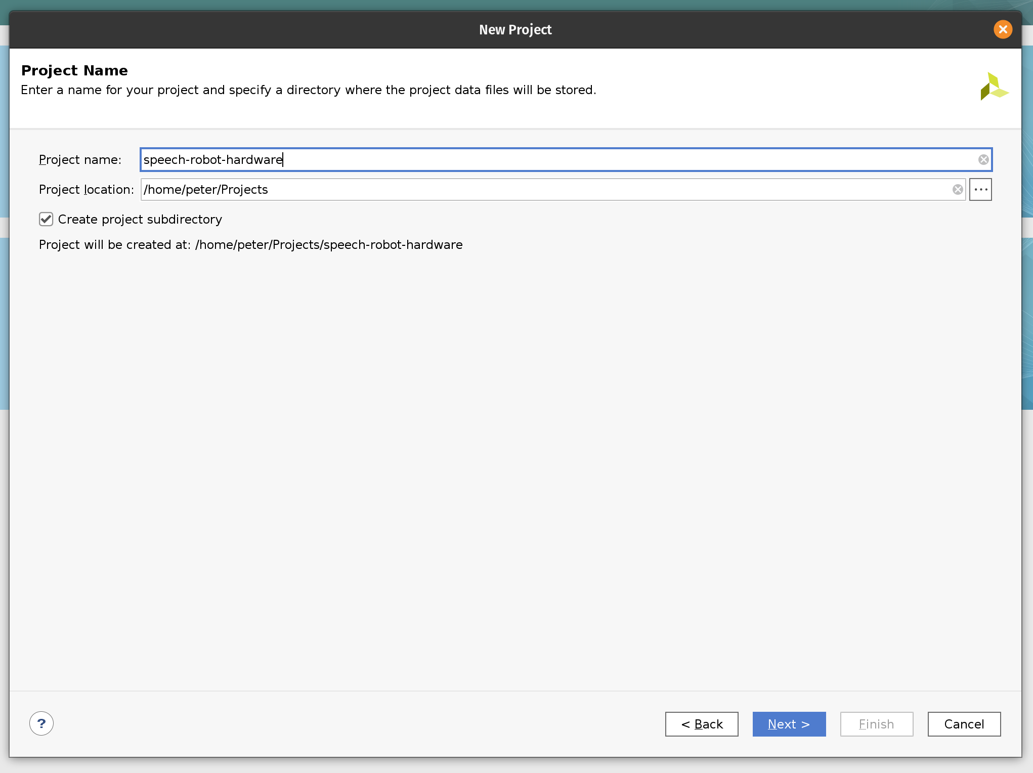
We start by creating a new Vivado project. Let’s name it speech-robot-hardware.
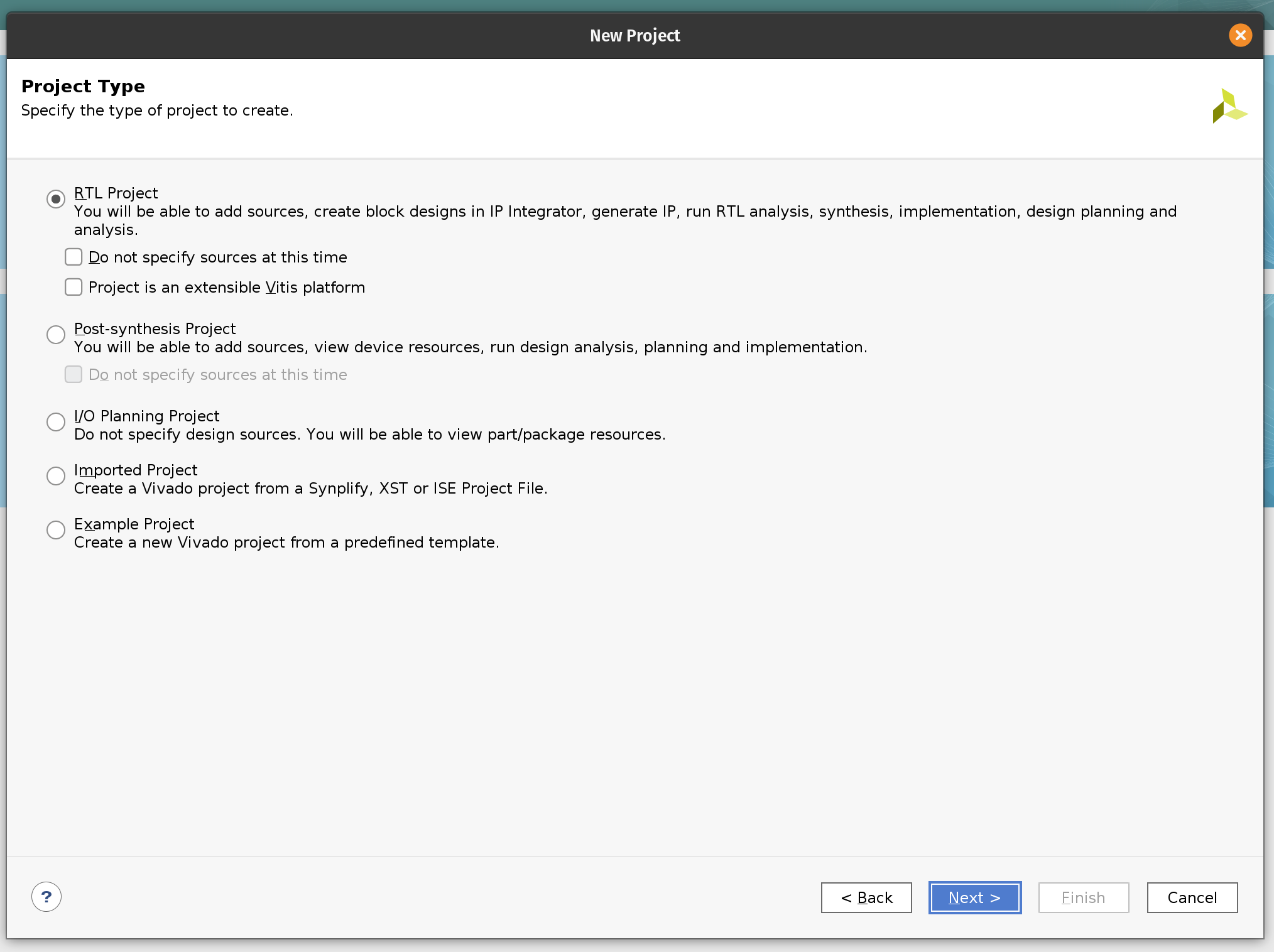
Next, we select the project type to be an RTL project.
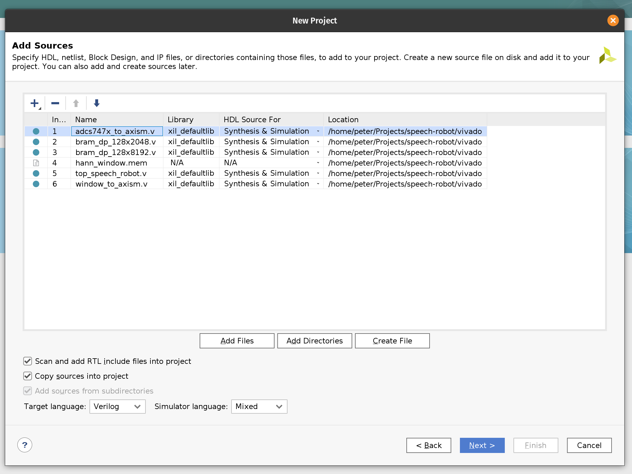
On the next page, add Verilog files and the hann_window.mem file with ROM content for the Hann window function.
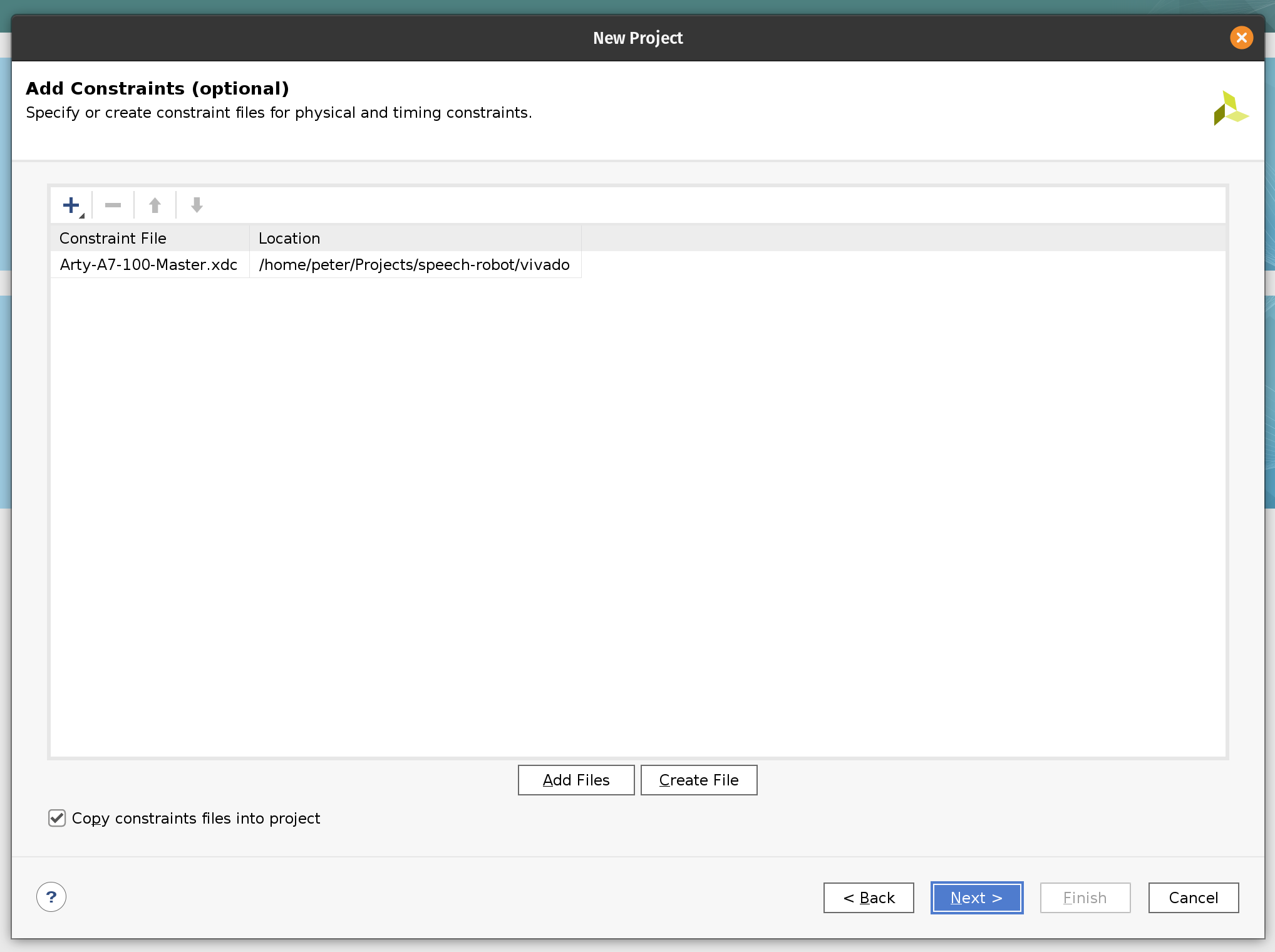
Next, add the Arty-A7-100-Master.xdc constraint file. We use this constraint file to assign the pins of the FPGA chip. The upper part of the JB PMOD interface is connected to the MIC3 module. The upper parts of the JA and JD PMOD interfaces are connected the left and right motor’s HB3 modules correspondingly.
The next page will allow us to select the target FPGA board. Search for “Arty” and select Arty A7-100. You may need to install the board definition by clicking on the icon in the Status column.
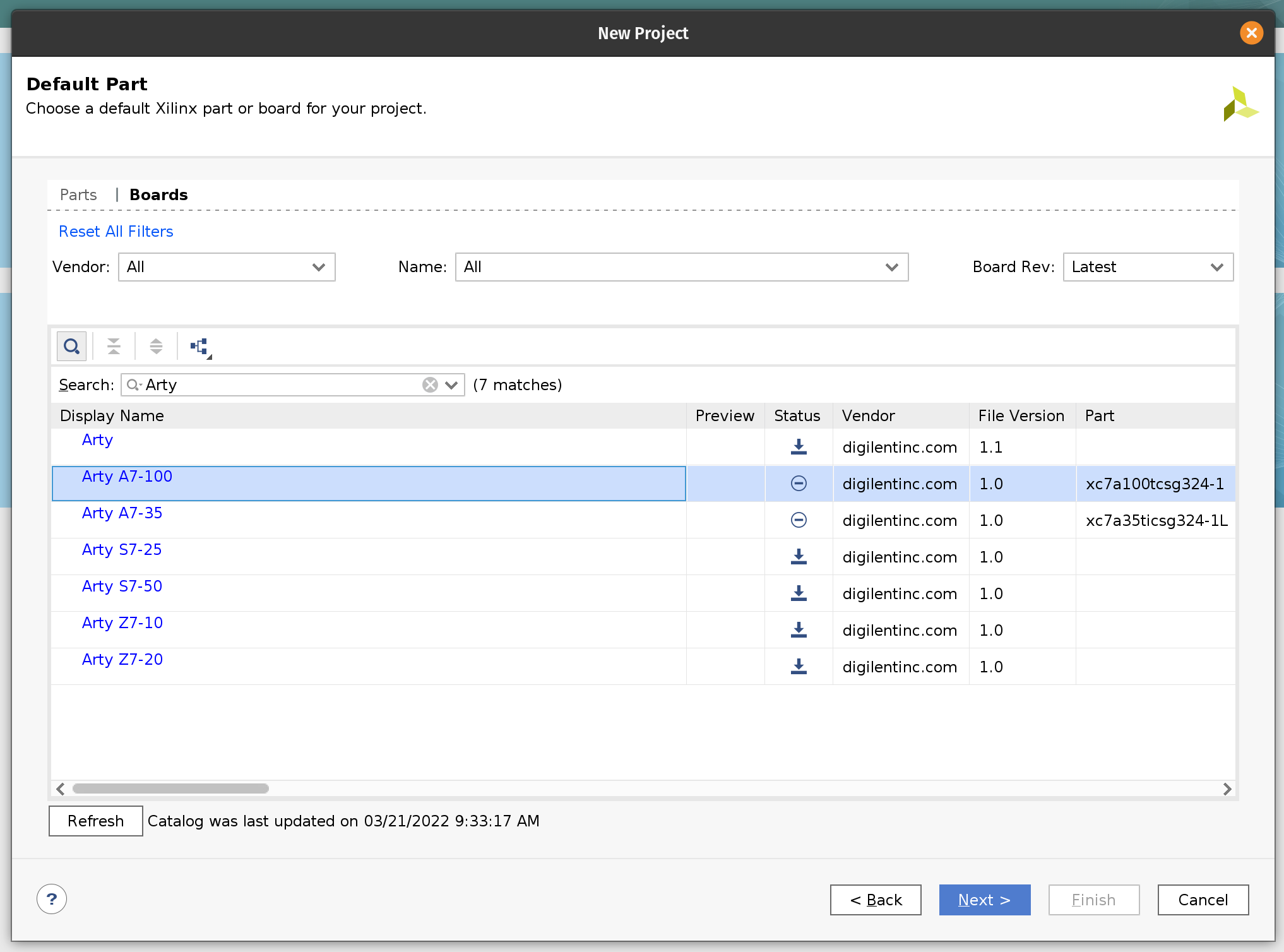
Click Next and Finish.
Next we need to import the Block Design. This will instantiate and configure the RTL we imported and many standard Xilinx components such as MicroBlaze, FFT and the DDR controller. The script then will wire everything together. In our previous Tensil tutorials we included step-by-step instructions on how to build Block Design from ground up. It was possible because the design was relatively simple. For the speech robot the design is a lot more complex. To save time we exported it from Vivado as a TCL script, which we now need to import.
To do this you will need to open the Vivado TCL console. (It should be one of the tabs at the bottom of the Vivado window.) Once in the console run the following command. Make sure to replace /home/peter/Projects/speech-robot with the path to the cloned GitHub repository.
source /home/peter/Projects/speech-robot/vivado/speech_robot.tcl
Once imported, right click on the speech_robot item in the Sources tab and then click on Create HDL Wrapper. Next choose to let Vivado manage wrapper and auto-update.
Once Vivado created the HDL wrapper the speech_robot item will get replaced with speech_robot_wrapper. Again, right click on it and then click Set as Top.
You should now be able to see the entire Block Design. (Image is clickable.)
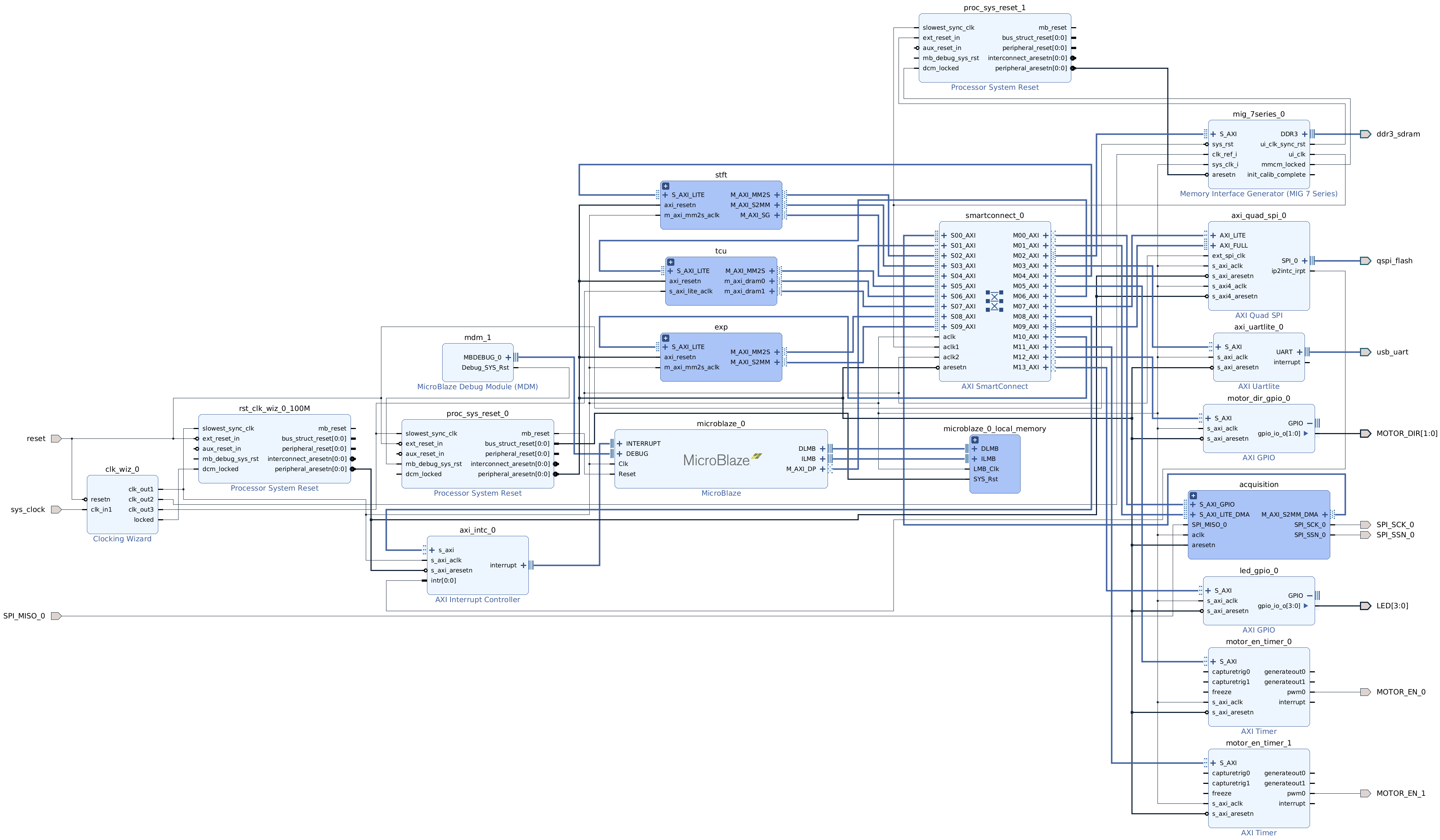
There are hierarchies (darker blue blocks) that correspond to our acceleration pipelines. These hierarchies are there to make the top-level diagram manageable. If you double-click on one of them they will open as a separate diagram. You can see that what is inside closely resembles diagrams from the discussion in the previous chapter.
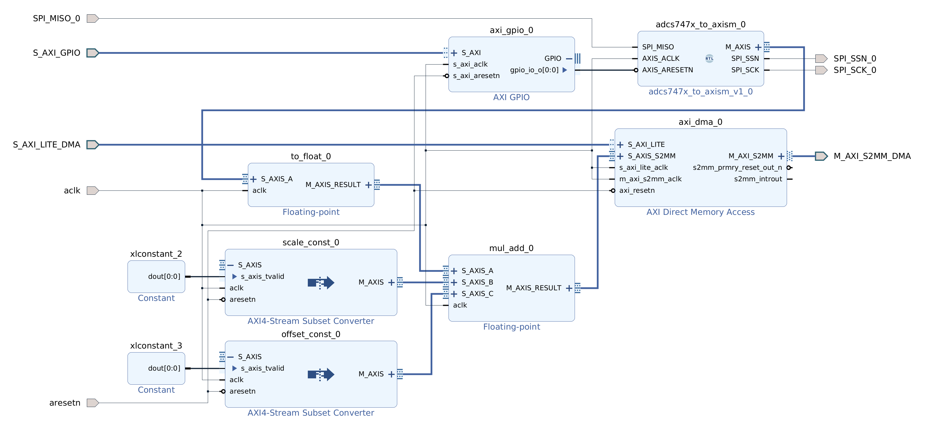
Let’s peek into the STFT pipeline. You can see Hann window multiplication on the left, followed by the Xilinx FFT component in the middle, followed by the magnitude and fixed point conversion operations on the right.

Similarly for acquisition and exponent pipelines.

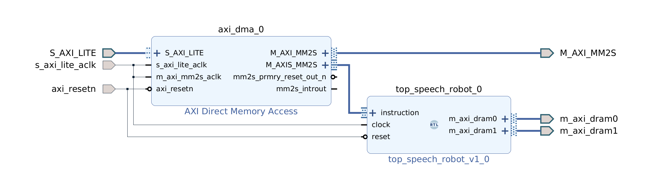
Design for the TCU hierarchy is very simple. We need an AXI DMA component to feed the program to the AXI4-Stream instruction port. DRAM0 and DRAM1 are full AXI ports and therefore go directly to the interconnect.
Now it’s time to synthesize the hardware. In the left-most pane click on Generate Bitstream, then click Yes and OK to launch the run. Now is a good time for a break!
Once Vivado finishes its run, the last step is to create the XSA file. Click on the File menu and then click Export and Export Hardware. Make sure that the XSA file includes the bitstream.
If you would like to skip the Vivado steps we included the XSA file in the GitHub repository.
Vitis embedded application
In this section we will follow the steps to build the software for the speech robot. We will use the Tensil embedded driver to interact with the TCU and the Xilinx AXI DMA driver to interact with other acceleration pipelines.
The entire application is contained in a single source code file. The comments contain further details that are not covered here. We highly recommend browsing through this file so that the rest of the tutorial makes more sense.
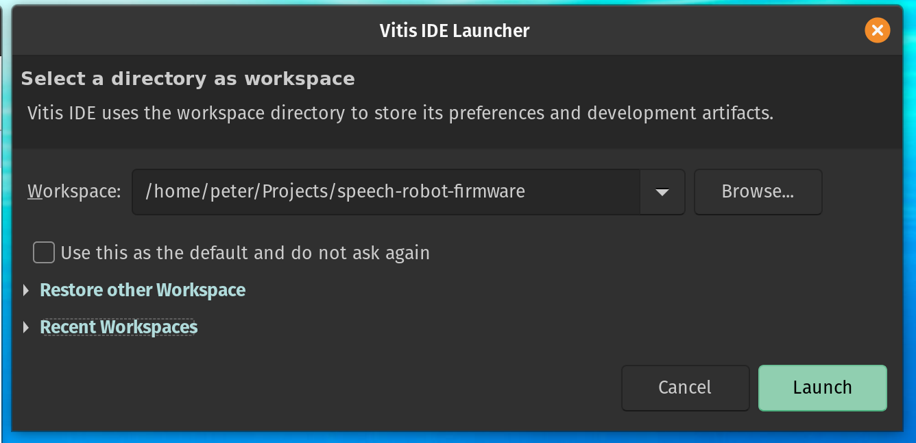
Let’s start by launching the Vitis IDE which prompts us to create a new workspace. Lets call it speech-robot-firmware.
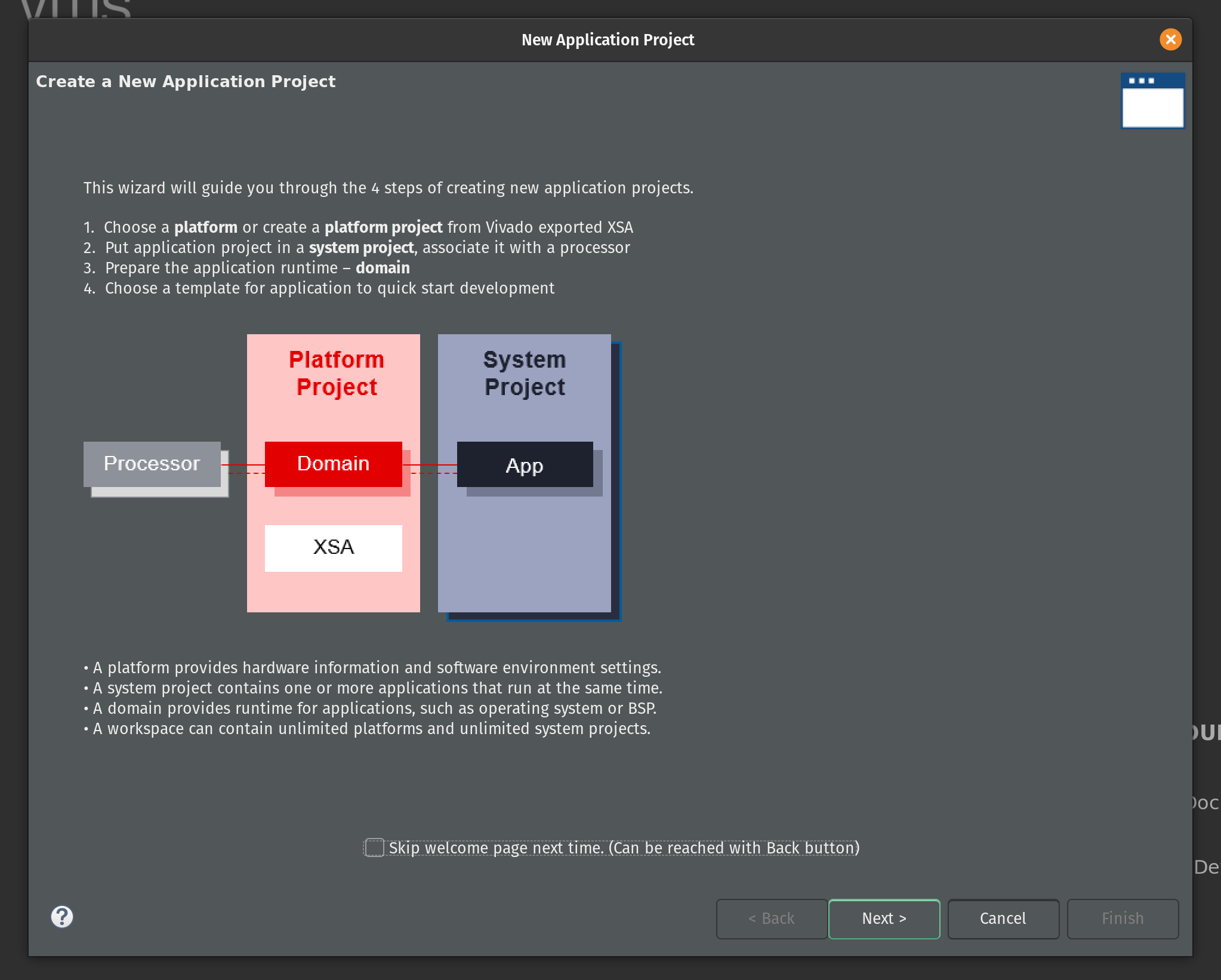
On the Vitis welcome page click Create Application Project. The first page of the New Application Project wizard explains what is going to happen. Click Next.
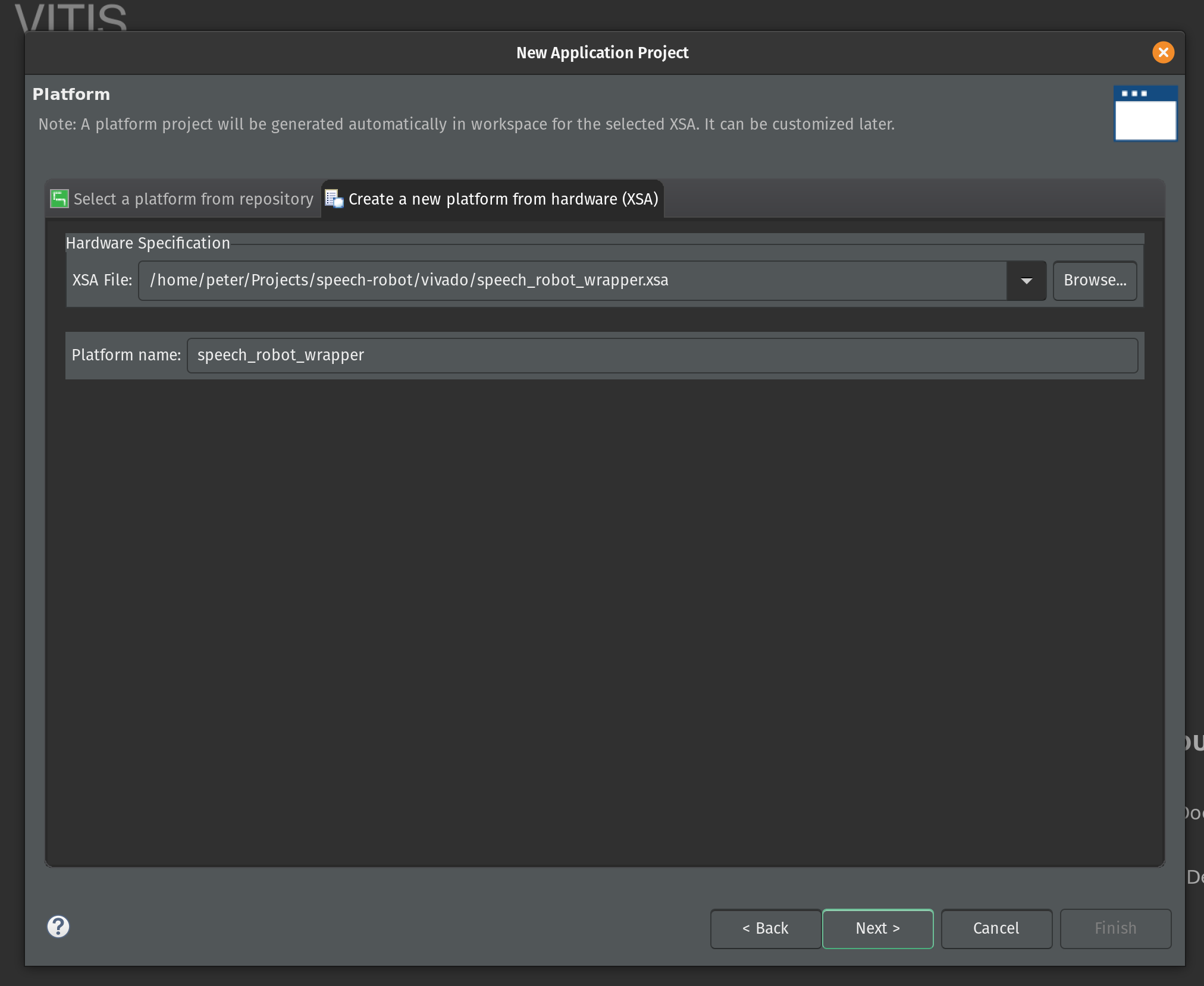
Now select Create a new platform from hardware (XSA) and select the location of the XSA file. Click Next.
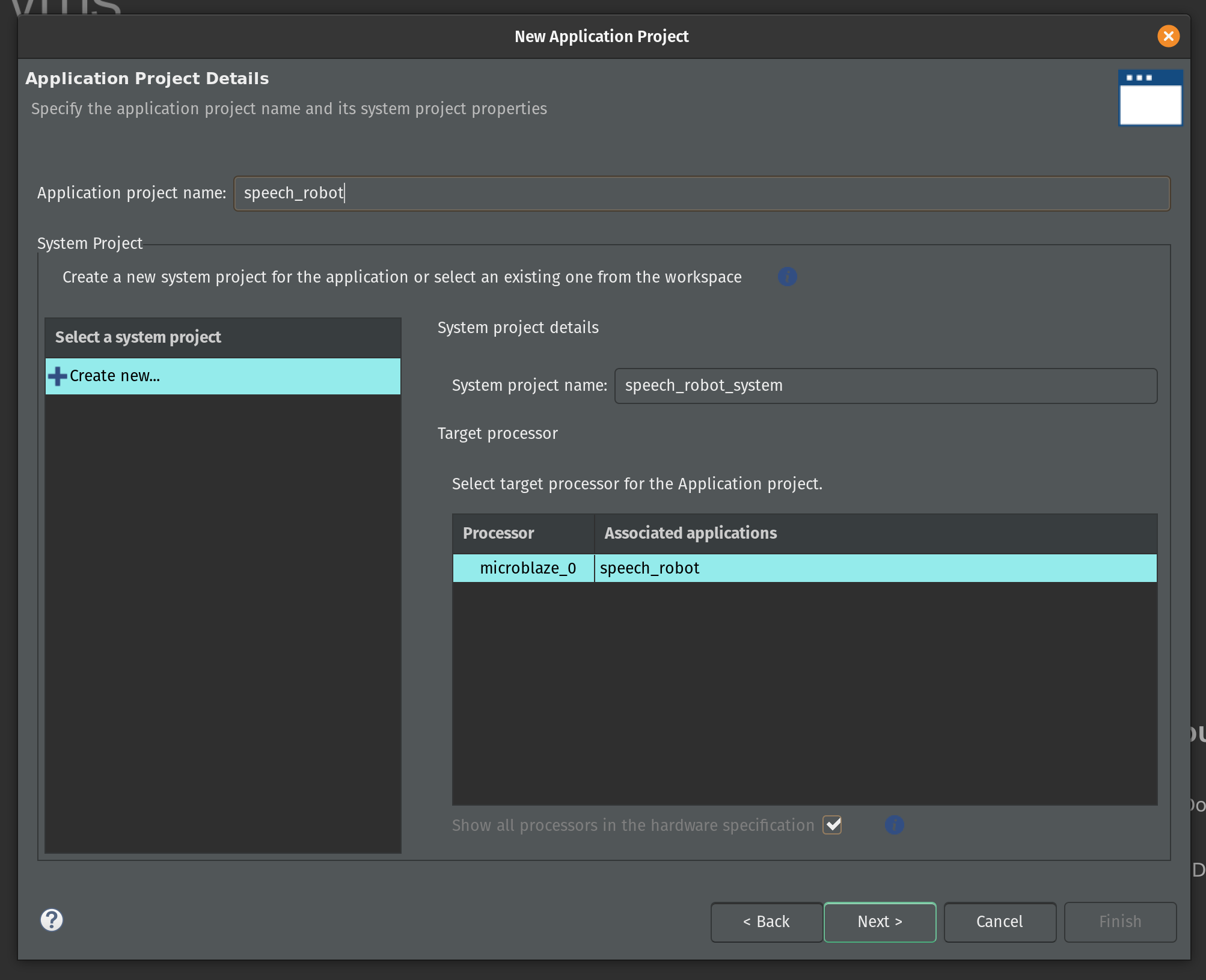
Enter the name for the application project. Type in speech_robot and click Next.
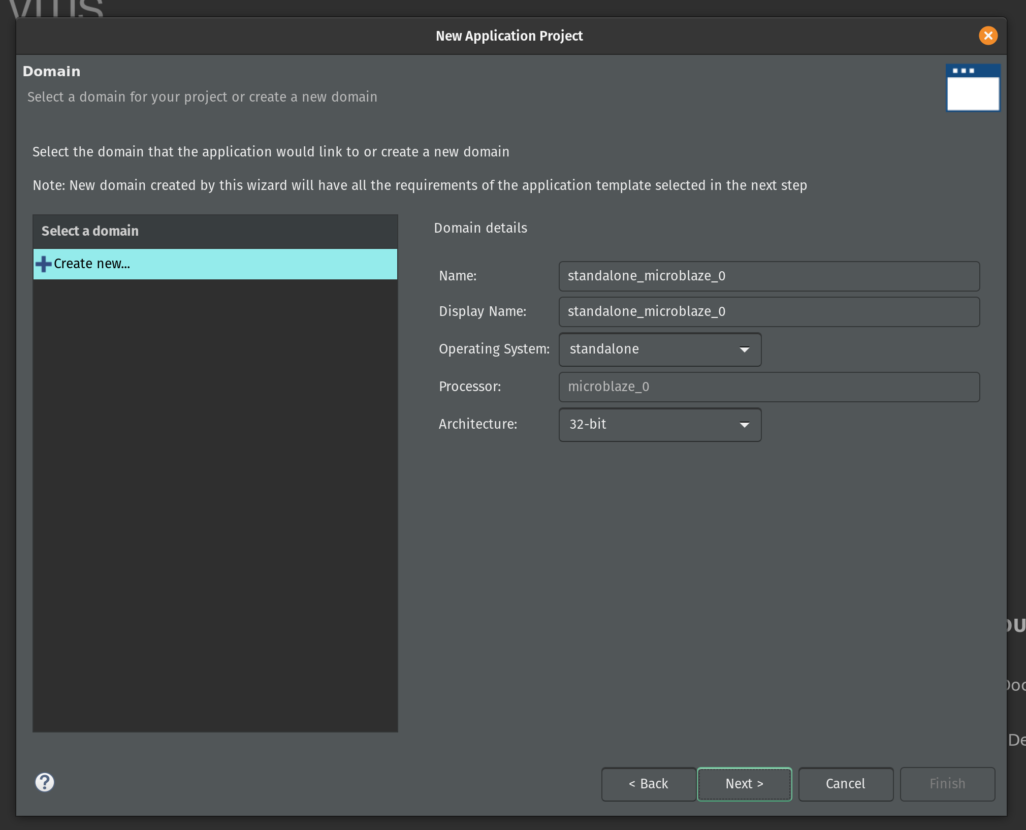
On the next page keep the default domain details unchanged and click Next.
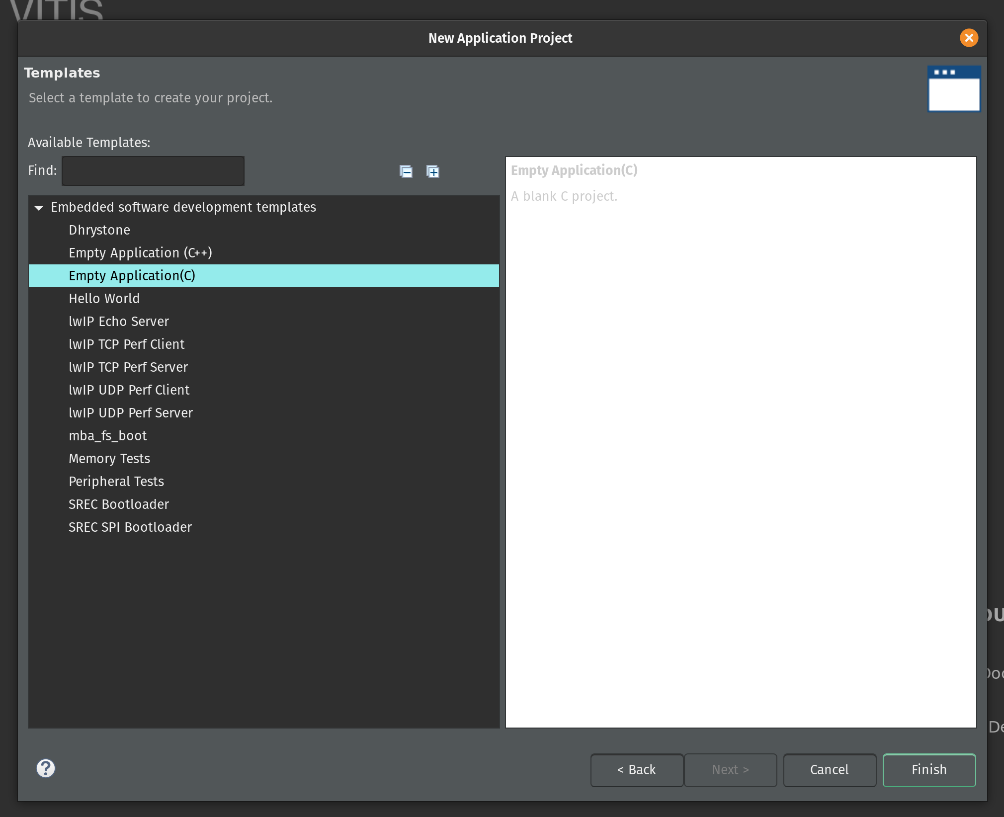
Select the Empty Application (C) as a template and click Finish.
Vitis created two projects in our workspace. The speech_robot_wrapper is a platform project that contains drivers and other base libraries configured for our specific hardware. This project is based on the XSA file and every time we change the XSA in Vivado we will need to update and rebuild the platform project.
The second is the system project speech_robot_system. The system project exposes tools to create boot images and program flash. (We’ll use Vivado for these functions instead.) The system project has an application subproject speech_robot. This project is what we will be populating with source files and building.
Let’s start by copying the source code for speech robot from its GitHub repository. The following commands assume that this repository and the Vitis workspace are on the same level in the file system.
cp speech-robot/vitis/speech_robot.c speech-robot-firmware/speech_robot/src/
cp speech-robot/vitis/lscript.ld speech-robot-firmware/speech_robot/src/
cp speech-robot/vivado/architecture_params.h speech-robot-firmware/speech_robot/src/
Next we need to clone Tensil repository and copy the embedded driver source code.
git clone [https://github.com/tensil-ai/tensil](https://github.com/tensil-ai/tensil)
cp -r tensil/drivers/embedded/tensil/ speech-robot-firmware/speech_robot/src/
Finally we copy one last file from the speech robot GitHub repository that will override the default Tensil platform definition.
cp speech-robot/vitis/tensil/platform.h speech-robot-firmware/speech_robot/src/tensil/
Now that we have all source files in the right places lets compile and link our embedded application. In the Assistant window in the left bottom corner click on Release under speech_robot [Application] project and then click Build.
This will generate an executable ELF file located in speech_robot/Release/speech_robot.elf under the Vitis workspace directory.
If you would like to skip the Vitis steps we included the ELF file in the GitHub repository.
Quad-SPI flash image
We now built both hardware (in the form of Vivado bitstream) and software (in the form of ELF executable file.) In this second to final section we will be combining them together with ML model artifacts to create the binary image for the flash memory.
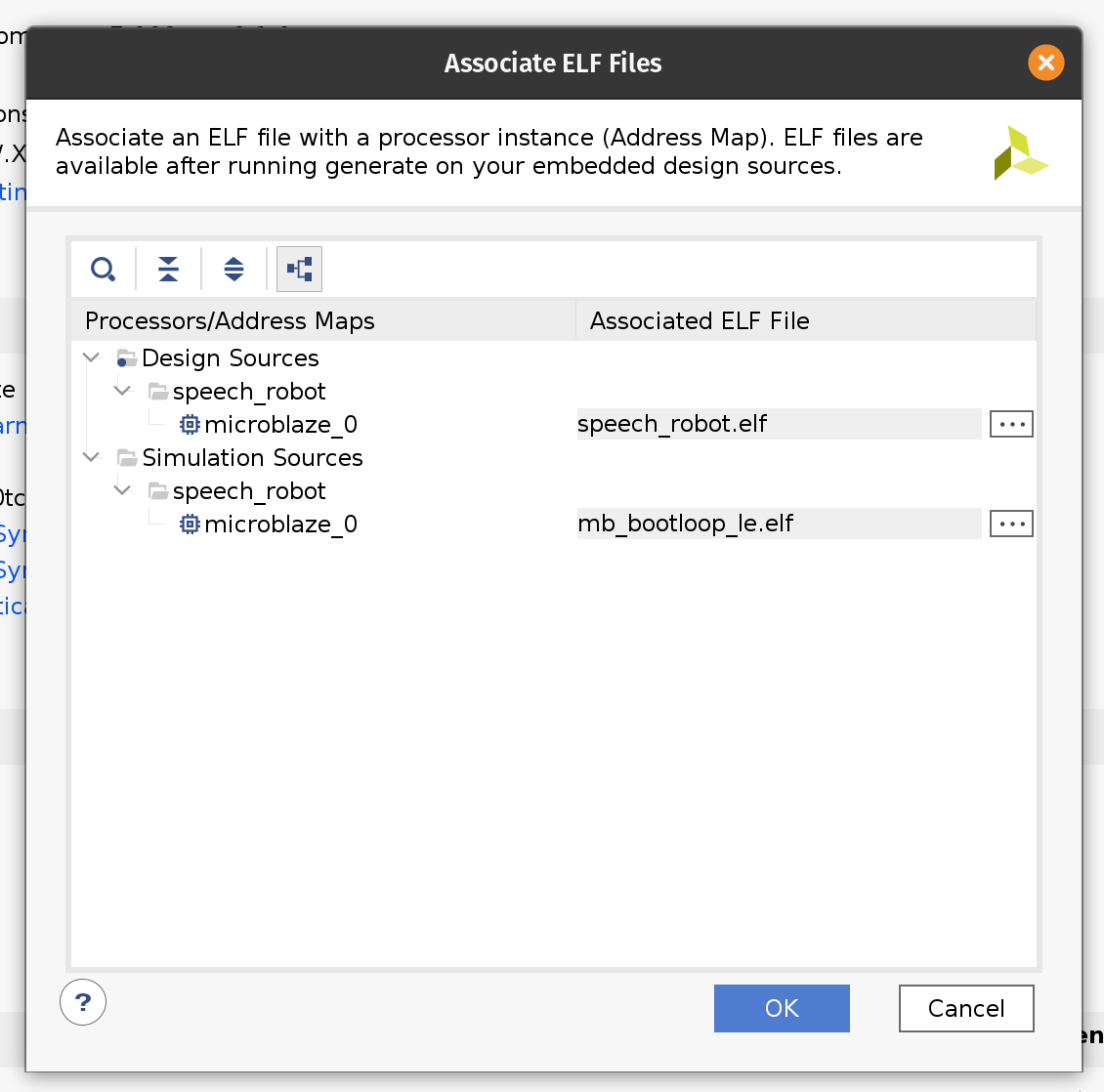
Firstly we need to update the bitstream with an ELF file containing our firmware. By default Vivado fills the Microblaze local memory with the default bootloader. To replace it go to the Tools menu and click Associate ELF files. Then click on the button with three dots and add the ELF file we produced in the previous section. Select it and click OK. Then click OK again.
Now that we changed the ELF file we need to rebuild the bitstream. Click the familiar Generate Bitstream in the left-side pane and wait for the run to complete.
Now we have a new bitstream file that has our firmware baked in!
Plug the Arty board into USB on your computer and then click Open Target under Open Hardware Manager and select Auto Connect.
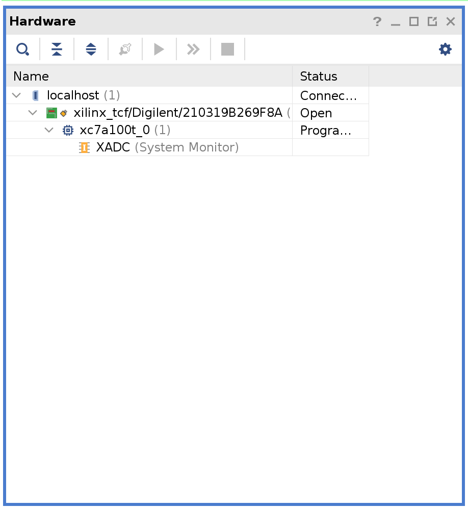
Right-click on xc7a100t_0 and then click Add Configuration Memory Device. Search for s25fl128sxxxxxx0 and select the found part and click OK.
If prompted to program the configuration memory device, click Cancel.
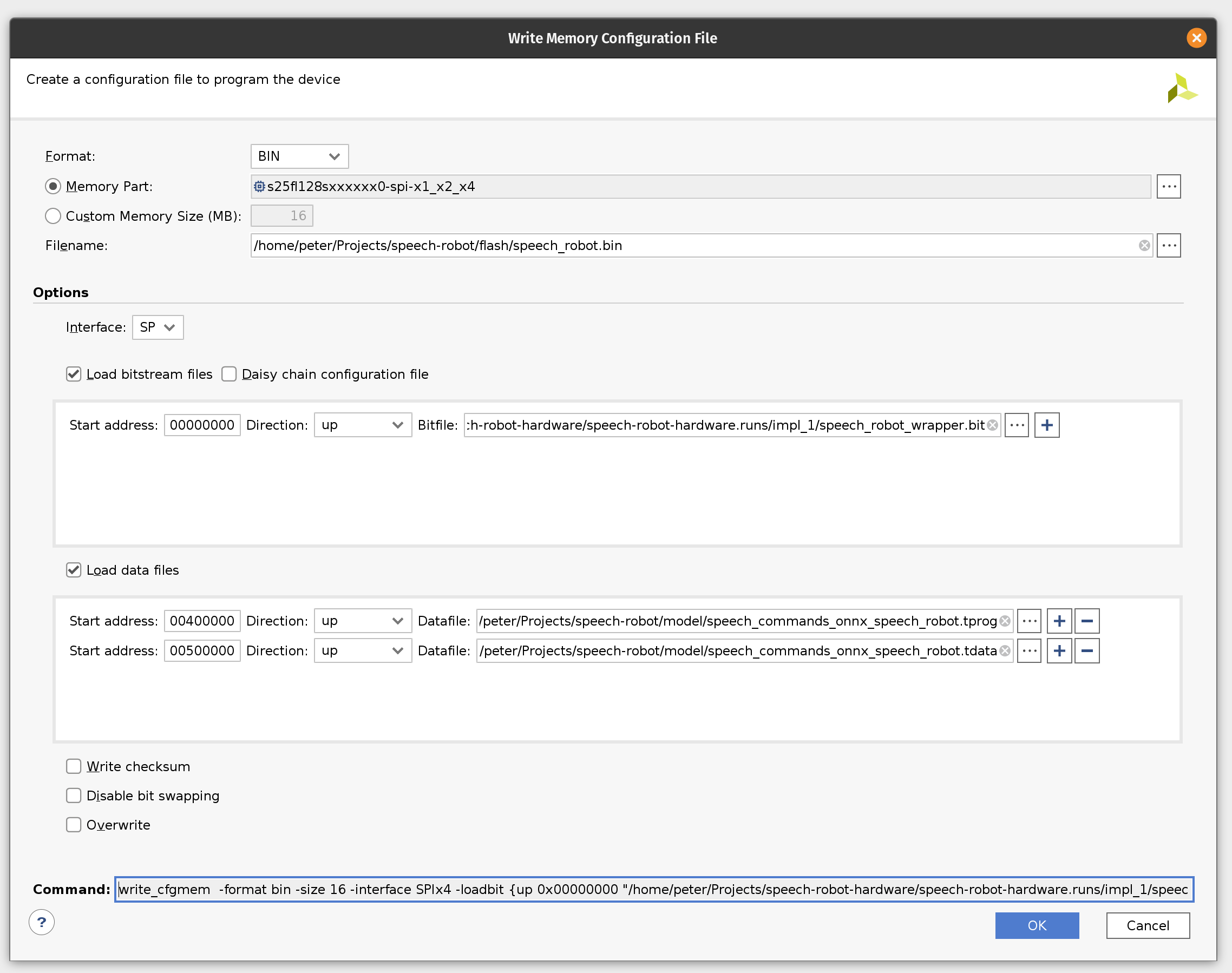
Click on the Tools menu and then click Generate Memory Configuration file. Choose the BIN format and select the available memory part. Enter filename for the flash memory image. (If you are overwriting the existing file, click the Overwrite checkbox at the bottom.)
Next, select the SPIx4 interface. Check the Load bitstream files and enter the location of the bitstream file. (It should be contained in speech-robot-hardware.runs/impl_1/ under the Vivado project directory.
Next, check the Load data files. Set the start address to 00400000 and enter the location of speech_commands_onnx_speech_robot.tprog file. Then click the plus icon. Set the next start address to 00500000 and enter the location of the speech_commands_onnx_speech_robot.tdata file. (Both files should be under the model directory in the GitHub repository.)
Click OK to generate the flash image BIN file.
If you would like to skip all the way to programming we included the BIN file in the GitHub repository.
Programming
In this final (FINAL!!!) section we’ll program the Arty board flash memory and should be able to run the sensor pipeline. The sensor pipeline will print every prediction to the UART device exposed via USB.
Plug the Arty board into USB on your computer and then click Open Target under Open Hardware Manager and select Auto Connect.
If you skipped the previous section where we were creating the flash image BIN file you will need to add the configuration memory device in the Hardware Manager. To do this right-click on xc7a100t_0 and then click Add Configuration Memory Device. Search for s25fl128sxxxxxx0 and select the found part and click OK. If prompted to program the configuration memory device, click OK.
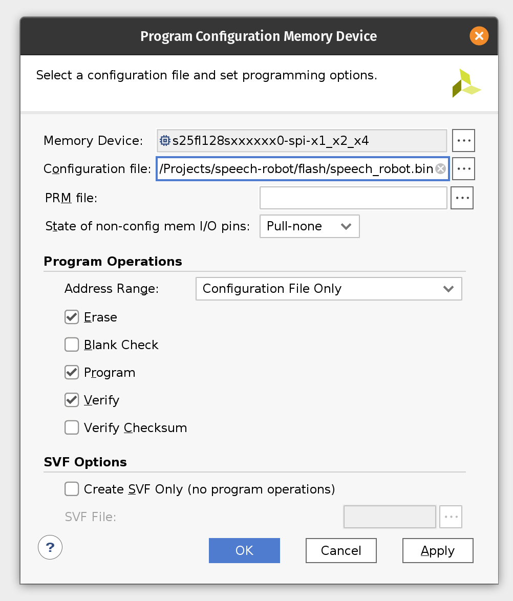
Otherwise right-click on s25fl128sxxxxxx0-spi-x1_x2_x4 and then click Program Configuration Memory Device. Enter the location of the flash image BIN file.
Click OK to program Arty flash.
Now make sure to close Vivado Hardware Manager, otherwise it will interfere with Arty booting from flash and disconnect the board from USB. Connect MIC3 module to the upper part of the JB PMOD interface.
Start the serial IO tool of your choice (like tio) and connect to /dev/ttyUSB1 at 115200 baud. It could be a different device depending on what else is plugged into your computer. Look for a device name starting with Future Technology Devices International.
tio -b 115200 /dev/ttyUSB1
Plug the Arty board back into USB and start shouting commands into your microphone!
The firmware will continuously print the latest prediction starting with its probability. When the event is handled by the State Machine it will add an arrow to highlight this.
0.986799860 _unknown_
0.598671191 _unknown_
0.317275269 up
0.884807667 _unknown_
0.894345367 _unknown_
0.660748154 go <<<
0.924147147 _unknown_
0.865093639 _unknown_
0.725528655 _silence_
0.959776973 _silence_
0.999572298 _silence_
0.993321552 _silence_
0.814953217 _unknown_
0.999999964 left <<<
0.999999981 left
0.999330031 _silence_
0.957002786 _silence_
0.704546136 _unknown_
0.913633790 right <<<
0.974430744 right
0.995242088 right
0.960198592 _silence_
0.870040107 _silence_
0.556416329 stop
0.919281920 _silence_
0.982788728 stop <<<
0.999821720 _silence_
0.913016908 _silence_
0.797638716 _silence_
0.610615039 _unknown_
0.623989887 _unknown_
Conclusion
In the part I of this tutorial we learned how to design an FPGA-based sensor pipeline that combines machine learning and digital signal processing (DSP). We used Tensil open source ML acceleration framework for ML part of the workload and the multitude of standard Xilinx components to implement DSP acceleration. Throughout the tutorial we saw Tensil work well in a very constrained environment of the Microblaze embedded application. Tensil’s entire driver along with the actual application fit in 64 KB of local Microblaze memory. We also saw Tensil integrate seamlessly with the standard Xilinx components, such as FFT, by using shared DDR memory, DMA and fixed point data type.
In part II we will learn how to design the state machine component of the robot and how to interface with motor drivers. Then we will switch from bits to atoms and integrate the Arty board and PMOD modules with the chassis, motors and on-board power distribution.
4 - Learn how to combine Tensil and TF-Lite to run YOLO on Ultra96
Originally posted here.
Introduction
This tutorial will use Avnet Ultra96 V2 development board and Tensil open-source inference accelerator to show how to run YOLO v4 Tiny–the state-of-the-art ML model for object detection–on FPGA. The YOLO model contains some operations that Tensil does not support. These operations are in the final stage of processing and are not compute-intensive. We will use TensorFlow Lite (TF-Lite) to run them on the CPU to work around this. We will use the PYNQ framework to receive real-time video from a USB webcam and show detected objects on a screen connected to Display Port. This tutorial refers to the previous Ultra96 tutorial for step-by-step instructions for generating Tensil RTL and getting Xilinx Vivado to synthesize the bitstream.
If you get stuck or find an error, you can ask a question on our Discord or send an email to [email protected].
Overview
Before we start, let’s get a bird’s eye view of what we want to accomplish. We’ll follow these steps:
- Generate and synthesize Tensil RTL
- Compile YOLO v4 Tiny model for Tensil
- Prepare PYNQ and TF-Lite
- Execute with PYNQ
1. Generate and synthesize Tensil RTL
In the first step, we’ll be getting Tensil tools to generate the RTL code and then using Xilinx Vivado to synthesize the bitstream for the Ultra96 board. Since this process is identical to other Ultra96 tutorials, we refer you to sections 1 through 4 in the ResNet20 tutorial.
Alternatively, you can skip this step and download the ready made bitstream. For this we include instructions in the subsequent section.
2. Compile YOLO v4 Tiny model for Tensil
Now, we need to compile the ML model to a Tensil binary consisting of TCU instructions executed by the TCU hardware directly. The YOLO v4 Tiny model is included in two resolutions, 192 and 416, in the Tensil docker image at /demo/models/yolov4_tiny_192.onnx and /demo/models/yolov4_tiny_416.onnx. The higher resolution will detect smaller objects using more computation and thus have fewer frames per second. Note that below we will be using 192 resolution, but simply replacing it with 416 should work as well.
As we mentioned in the introduction, we will be using the TF-Lite framework to run the postprocessing of YOLO v4 Tiny. Specifically, this postprocessing includes Sigmoid and Exp operations not supported by the Tensil hardware. (We plan to implement them using table lookup based on Taylor expansion.) This means that for Tensil we need to compile the model ending with the last convolution layers. Below these layers, we need to compile the TF-Lite model. To identify the output nodes for the Tensil compiler, take a look at the model in Netron.
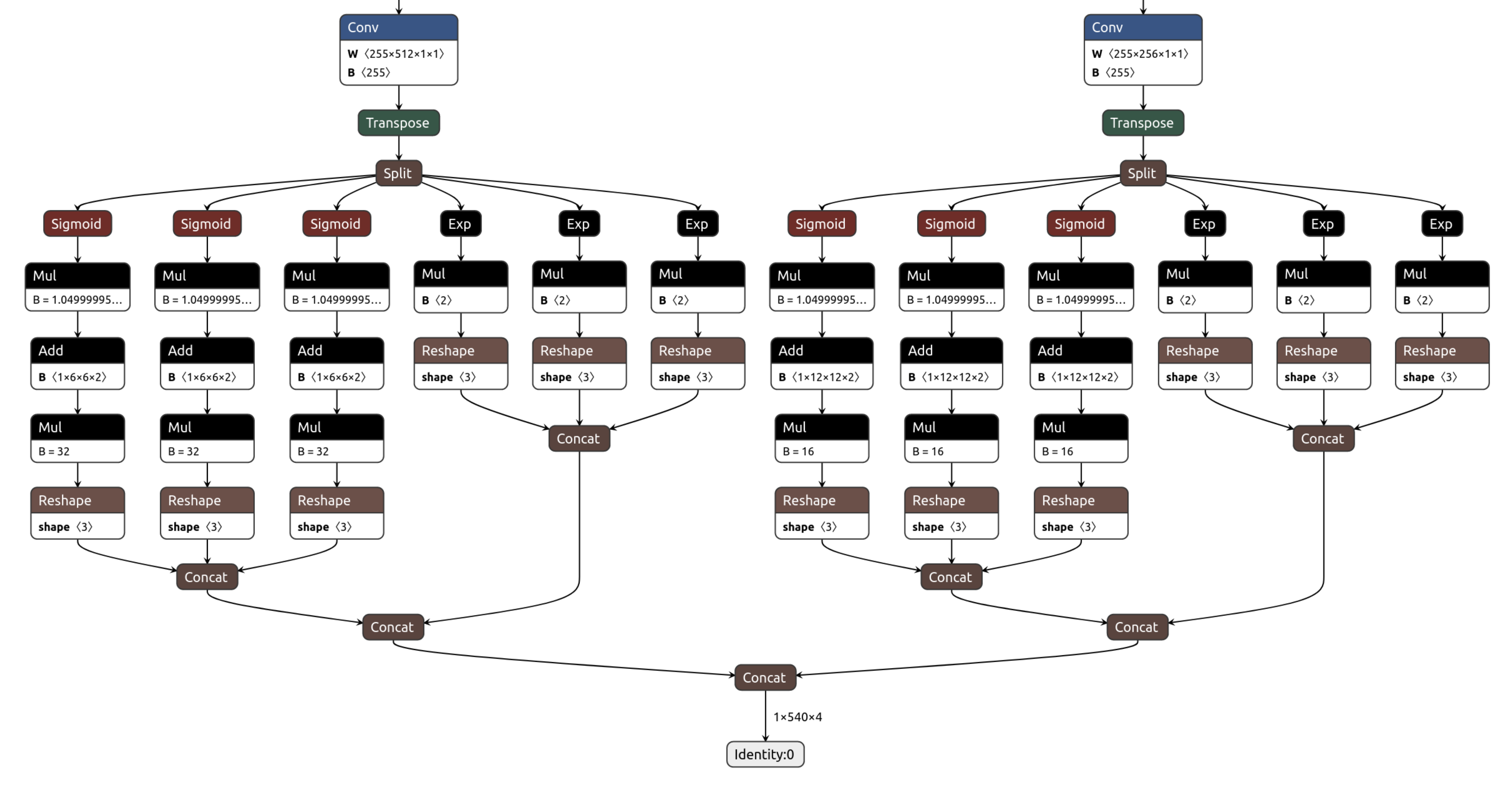
Two last convolution operation have outputs named model/conv2d_17/BiasAdd:0 and model/conv2d_20/BiasAdd:0.
From within the Tensil docker container, run the following command.
tensil compile -a /demo/arch/ultra96v2.tarch -m /demo/models/yolov4_tiny_192.onnx -o "model/conv2d_17/BiasAdd:0,model/conv2d_20/BiasAdd:0" -s true
The resulting compiled files are listed in the ARTIFACTS table. The manifest (tmodel) is a plain text JSON description of the compiled model. The Tensil program (tprog) and weights data (tdata) are both binaries to be used by the TCU during execution. The Tensil compiler also prints a COMPILER SUMMARY table with interesting stats for both the TCU architecture and the model.
---------------------------------------------------------------------------------------------
COMPILER SUMMARY
---------------------------------------------------------------------------------------------
Model:                                           yolov4_tiny_192_onnx_ultra96v2
Data type:                                       FP16BP8
Array size:                                      16
Consts memory size (vectors/scalars/bits):       2,097,152                      33,554,432 21
Vars memory size (vectors/scalars/bits):         2,097,152                      33,554,432 21
Local memory size (vectors/scalars/bits):        20,480                         327,680    15
Accumulator memory size (vectors/scalars/bits):  4,096                          65,536     12
Stride #0 size (bits):                           3
Stride #1 size (bits):                           3
Operand #0 size (bits):                          24
Operand #1 size (bits):                          24
Operand #2 size (bits):                          16
Instruction size (bytes):                        9
Consts memory maximum usage (vectors/scalars):   378,669                        6,058,704
Vars memory maximum usage (vectors/scalars):     55,296                         884,736
Consts memory aggregate usage (vectors/scalars): 378,669                        6,058,704
Vars memory aggregate usage (vectors/scalars):   130,464                        2,087,424
Number of layers:                                25
Total number of instructions:                    691,681
Compilation time (seconds):                      92.225
True consts scalar size:                         6,054,190
Consts utilization (%):                          98.706
True MACs (M):                                   670.349
MAC efficiency (%):                              0.000
---------------------------------------------------------------------------------------------
3. Prepare PYNQ and TF-Lite
Now it’s time to put everything together on our development board. For this, we first need to set up the PYNQ environment. This process starts with downloading the SD card image for our development board. There’s the detailed instruction for setting board connectivity on the PYNQ documentation website. You should be able to open Jupyter notebooks and run some examples. Note that you’ll need wireless internet connectivity for your Ultra96 board in order to run some of the commands in this section.
There is one caveat that needs addressing once PYNQ is installed. On the default PYNQ image, the setting for the Linux kernel CMA (Contiguous Memory Allocator) area size is 128MB. Given our Tensil architecture, the default CMA size is too small. To address this, you’ll need to download our patched kernel, copy it to /boot, and reboot your board. Note that the patched kernel is built for PYNQ 2.7 and will not work with other versions. To patch the kernel, run these commands on the development board:
wget https://s3.us-west-1.amazonaws.com/downloads.tensil.ai/pynq/2.7/ultra96v2/image.ub
sudo cp /boot/image.ub /boot/image.ub.backup
sudo cp image.ub /boot/
rm image.ub
sudo reboot
Now that PYNQ is up and running, the next step is to scp the Tensil driver for PYNQ. Start by cloning the Tensil GitHub repository to your work station and then copy drivers/tcu_pynq to /home/xilinx/tcu_pynq onto your board.
git clone [email protected]:tensil-ai/tensil.git
scp -r tensil/drivers/tcu_pynq [email protected]:
Next, we’ll download the bitstream created for Ultra96 architecture definition we used with the compiler. The bitstream contains the FPGA configuration resulting from Vivado synthesis and implementation. PYNQ also needs a hardware handoff file that describes FPGA components accessible to the host, such as DMA. Download and un-tar both files in /home/xilinx by running these commands on the development board.
wget https://s3.us-west-1.amazonaws.com/downloads.tensil.ai/hardware/1.0.4/tensil_ultra96v2.tar.gz
tar -xvf tensil_ultra96v2.tar.gz
If you’d like to explore using Tensil RTL tool and Xilinx Vivado to synthesize the bitstream yourself, we refer you to sections 1 through 4 in the ResNet20 tutorial. Section 6 in the same tutorial includes instructions for copying the bitstream and hardware handoff file from Vivado project onto your board.
Now, copy the .tmodel, .tprog and .tdata artifacts produced by the compiler on your work station to /home/xilinx on the board.
scp yolov4_tiny_192_onnx_ultra96v2.t* [email protected]:
Next, we need to set up TF-Lite. We prepared the TF-Lite build compatible with the Ultra96 board. Run the following commands on the development board to download and install.
wget https://s3.us-west-1.amazonaws.com/downloads.tensil.ai/tflite_runtime-2.8.0-cp38-cp38-linux_aarch64.whl
sudo pip install tflite_runtime-2.8.0-cp38-cp38-linux_aarch64.whl
Finally, we will need the TF-Lite model to run the postprocessing in YOLO v4 Tiny. We prepared this model for you as well. We’ll also need text labels for the COCO dataset used for training the YOLO model. Download these files into /home/xilinx by running these commands on the development board.
wget https://github.com/tensil-ai/tensil-models/raw/main/yolov4_tiny_192_post.tflite
wget https://raw.githubusercontent.com/amikelive/coco-labels/master/coco-labels-2014_2017.txt
4. Execute with PYNQ
Now, we will be tying everything together in PYNQ Jupyter notebook. Let’s take a closer look at our processing pipeline.
- Capture the frame image from the webcam;
- Adjust the image size, color scheme, floating-point channel representation, and Tensil vector alignment to match YOLO v4 Tiny input;
- Run it through Tensil to get the results of the two final convolution layers;
- Subsequently run these results through the TF-Lite interpreter to get the model output for bounding boxes and classification scores;
- Filter bounding boxes based on the score threshold and suppress overlapping boxes for the same detected object;
- Use the frame originally captured from the camera to plot bounding boxes, class names, scores (red), the current value for frames per second (green), and the detection area (blue);
- Send this annotated frame to Display Port to show on the screen.
At the beginning of the notebook, we define global parameters: frame dimensions for both camera and screen and YOLO v4 Tiny resolution we will be using.
model_hw = 192
frame_w = 1280
frame_h = 720
Next, we import the Tensil PYNQ driver and other required utilities.
import sys
sys.path.append('/home/xilinx/')

import time
import math
import numpy as np
import tflite_runtime.interpreter as tflite
import cv2
import matplotlib.pyplot as plt
import pynq

from pynq import Overlay
from pynq.lib.video import *

from tcu_pynq.driver import Driver
from tcu_pynq.util import div_ceil
from tcu_pynq.architecture import ultra96
Now, initialize the PYNQ overlay from the bitstream and instantiate the Tensil driver using the TCU architecture and the overlay’s DMA configuration. Note that we are passing axi_dma_0 object from the overlay–the name matches the DMA block in the Vivado design.
overlay = Overlay('/home/xilinx/tensil_ultra96v2.bit')
tcu = Driver(ultra96, overlay.axi_dma_0)
Next, we need to initialize the capture from the webcam using OpenCV library.
cap = cv2.VideoCapture(0)

cap.set(cv2.CAP_PROP_FRAME_WIDTH, frame_w);
cap.set(cv2.CAP_PROP_FRAME_HEIGHT, frame_h);
And initialze the Dispay Port.
displayport = DisplayPort()
displayport.configure(VideoMode(frame_w, frame_h, 24), PIXEL_RGB)
If you are connecting the board to an HDMI screen, make sure to use active DP-to-HDMI cable, such as this one.
Next, load the tmodel manifest for the model into the driver. The manifest tells the driver where to find the other two binary files (program and weights data).
tcu.load_model('/home/xilinx/yolov4_tiny_{0}_onnx_ultra96v2.tmodel'.format(model_hw))
Then, instantiate the TF-Lite interpreter based on YOLO postprocessing model.
interpreter = tflite.Interpreter(model_path='/home/xilinx/yolov4_tiny_{0}_post.tflite'.format(model_hw))
interpreter.allocate_tensors()
Now we load the COCO labels and define several utility functions.
with open('/home/xilinx/coco-labels-2014_2017.txt') as f:
    labels_coco = f.read().split('\n')

def set_tensor(driver, interpreter, hw_size, data):
    input_details = interpreter.get_input_details()
    input_idxs = [i for i in range(len(input_details))
                  if input_details[i]['shape'][1] == hw_size and input_details[i]['shape'][2] == hw_size]
    inp = input_details[input_idxs[0]]
    data = data.astype(inp['dtype'])
    inner_dim = inp['shape'][-1]
    inner_size = div_ceil(inner_dim, driver.arch.array_size) * driver.arch.array_size
    if inner_size != inner_dim:
        data = data.reshape((-1, inner_size))[:, :inner_dim]
    data = data.reshape(inp['shape'])
    interpreter.set_tensor(inp['index'], data)

def filter_and_reshape(boxes, scores, score_threshold=0.4):
    scores_max = np.max(scores, axis=-1)
    mask = scores_max > score_threshold

    filtered_boxes = boxes[mask]
    filtered_scores = scores[mask]

    filtered_boxes = np.reshape(filtered_boxes, [scores.shape[0], -1, filtered_boxes.shape[-1]])
    filtered_scores = np.reshape(filtered_scores, [scores.shape[0], -1, filtered_scores.shape[-1]])

    return filtered_boxes, filtered_scores


def non_maximum_suppression(boxes, iou_threshold=0.4):
    if len(boxes) == 0:
        return boxes

    area = (boxes[:, 2] - boxes[:, 0]) * (boxes[:, 3] - boxes[:, 1])
    ll_x = np.maximum.outer(boxes[:, 0], boxes[:, 0])
    ll_y = np.maximum.outer(boxes[:, 1], boxes[:, 1])
    ur_x = np.minimum.outer(boxes[:, 2], boxes[:, 2])
    ur_y = np.minimum.outer(boxes[:, 3], boxes[:, 3])
    intersection_x = np.maximum(0, ur_x - ll_x)
    intersection_y = np.maximum(0, ur_y - ll_y)
    intersection = intersection_x * intersection_y

    iou = intersection / area - np.identity(area.shape[-1])
    p = iou >= iou_threshold
    p = p & p.T
    n =  p.shape[-1]

    no_needs_merge = set()
    for i in range(n):
        if not p[i].any():
            no_needs_merge.add(i)

    needs_merge = set()
    for i in range(n):
        for j in range(n):
            if p[i, j]:
                needs_merge.add(tuple(sorted((i, j))))

    def merge(needs_merge):
        result = set()
        discarded = set()
        for indices in needs_merge:
            idx = indices[0]
            if idx not in discarded:
                result.add(indices[0])
            discarded.add(indices[1])
            if indices[1] in result:
                result.remove(indices[1])
        return result

    return sorted(list(no_needs_merge) + list(merge(needs_merge)))
Finally, we tie the pipeline together in a loop to process a fixed number of frames. (You may replace it with while(1): to run the pipeline indefinitely.)
for _ in range(600):
    start = time.time()

    cap_frame = displayport.newframe()
    cap.read(cap_frame)

    crop_h = int(max(0, (frame_h - frame_w) / 2))
    crop_w = int(max(0, (frame_w - frame_h) / 2))
    ratio_h = (frame_h - crop_h * 2)/model_hw
    ratio_w = (frame_w - crop_w * 2)/model_hw

    x_frame = cap_frame
    x_frame=x_frame[crop_h:frame_h - crop_h, crop_w:frame_w - crop_w]
    x_frame=cv2.resize(x_frame, (model_hw, model_hw), interpolation=cv2.INTER_LINEAR)
    x_frame=cv2.cvtColor(x_frame, cv2.COLOR_BGR2RGB)
    x_frame = x_frame.astype('float32') / 255
    x_frame = np.pad(x_frame, [(0, 0), (0, 0), (0, tcu.arch.array_size - 3)], 'constant', constant_values=0)

    inputs = {'x:0': x_frame}
    outputs = tcu.run(inputs)

    set_tensor(tcu, interpreter, model_hw / 32, np.array(outputs['model/conv2d_17/BiasAdd:0']))
    set_tensor(tcu, interpreter, model_hw / 16, np.array(outputs['model/conv2d_20/BiasAdd:0']))

    interpreter.invoke()

    output_details = interpreter.get_output_details()
    scores, boxes_xywh = [interpreter.get_tensor(output_details[i]['index']) for i in range(len(output_details))]

    boxes_xywh, scores = filter_and_reshape(boxes_xywh, scores)

    boxes_xy, boxes_wh = np.split(boxes_xywh, (2,), axis=-1)
    boxes_x0y0x1y1 = np.concatenate([boxes_xy - boxes_wh/2, boxes_xy + boxes_wh/2], axis=-1)

    box_indices = non_maximum_suppression(boxes_x0y0x1y1[0])

    latency = (time.time() - start)
    fps = 1/latency

    for i in box_indices:
        category_idx = np.argmax(scores, axis=-1)[0, i]
        category_conf = np.max(scores, axis=-1)[0, i]
        text = f'{labels_coco[category_idx]} = {category_conf:.2}'

        box_x0y0x1y1 = boxes_x0y0x1y1[0, i]
        box_x0y0x1y1[0] *= ratio_w
        box_x0y0x1y1[1] *= ratio_h
        box_x0y0x1y1[2] *= ratio_w
        box_x0y0x1y1[3] *= ratio_h
        box_x0y0x1y1[0] += crop_w
        box_x0y0x1y1[1] += crop_h
        box_x0y0x1y1[2] += crop_w
        box_x0y0x1y1[3] += crop_h
        box_x0y0x1y1 = box_x0y0x1y1.astype('int')

        cap_frame = cv2.rectangle(cap_frame, (crop_w, crop_h), (frame_w - crop_w, frame_h - crop_h), (255, 0, 0), 1)
        cap_frame = cv2.rectangle(cap_frame, (box_x0y0x1y1[0], box_x0y0x1y1[1]), (box_x0y0x1y1[2], box_x0y0x1y1[3]), (0, 0, 255), 1)
        cap_frame = cv2.putText(cap_frame, text, (box_x0y0x1y1[0] + 2, box_x0y0x1y1[1] - 2), cv2.FONT_HERSHEY_SIMPLEX, 0.75, (0, 0, 255))


    cap_frame = cv2.putText(cap_frame, f'{fps:.2}fps', (2, frame_h - 2), cv2.FONT_HERSHEY_SIMPLEX, 0.75, (0, 255, 0))
    displayport.writeframe(cap_frame)
After running the pipeline, we clean up the camera capture and Display Port resources.
displayport.close()
cap.release()
tcu.close()
Congratulations! You ran a state-of-the-art object detection ML model on a custom accelerator hooked to a webcam and a screen for real-time object detection! Just imagine the things you could do with it…
Wrap-up
In this tutorial we used Tensil to show how to run YOLO v4 Tiny ML model on FPGA with a postprocessing step handled by TF-Lite. We showed how to analyze the model to detemine the layers at which to split the processing between TF-Lite and Tensil. We included step-by-step explanation how to do real-time video processing pipeline using PYNQ.
If you made it all the way through, big congrats! You’re ready to take things to the next level by trying out your own model and architecture. Join us on Discord to say hello and ask questions, or send an email to [email protected].
5 - Learn Tensil with ResNet and PYNQ Z1
Originally posted here.
Introduction
This tutorial will use the PYNQ Z1 development board and Tensil’s open-source inference accelerator to show how to run machine learning (ML) models on FPGA. We will be using ResNet-20 trained on the CIFAR dataset. These steps should work for any supported ML model – currently all the common state-of-the-art convolutional neural networks are supported. Try it with your model!
We’ll give detailed end-to-end coverage that is easy to follow. In addition, we include in-depth explanations to get a good understanding of the technology behind it all, including the Tensil and Xilinx Vivado toolchains and PYNQ framework.
If you get stuck or find an error, you can ask a question on our Discord or send an email to [email protected].
Overview
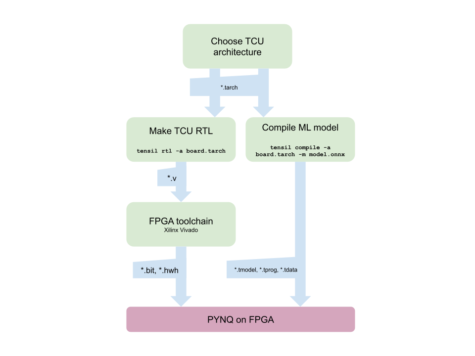
Before we start, let’s look at the Tensil toolchain flow to get a bird’s eye view of what we want to accomplish. We’ll follow these steps:
- Get Tensil
- Choose architecture
- Generate TCU accelerator design (RTL code)
- Synthesize for PYNQ Z1
- Compile ML model for TCU
- Execute using PYNQ
1. Get Tensil
First, we need to get the Tensil toolchain. The easiest way is to pull the Tensil docker container from Docker Hub. The following command will pull the image and then run the container.
docker pull tensilai/tensil
docker run -v $(pwd):/work -w /work -it tensilai/tensil bash
2. Choose architecture
Tensil’s strength is customizability, making it suitable for a very wide range of applications. The Tensil architecture definition file (.tarch) specifies the parameters of the architecture to be implemented. These parameters are what make Tensil flexible enough to work for small embedded FPGAs as well as large data-center FPGAs. Our example will select parameters that provide the highest utilization of resources on the XC7Z020 FPGA part at the core of the PYNQ Z1 board. The container image conveniently includes the architecture file for the PYNQ Z1 development board at /demo/arch/pynqz1.tarch. Let’s take a look at what’s inside.
{
    "data_type": "FP16BP8",
    "array_size": 8,
    "dram0_depth": 1048576,
    "dram1_depth": 1048576,
    "local_depth": 8192,
    "accumulator_depth": 2048,
    "simd_registers_depth": 1,
    "stride0_depth": 8,
    "stride1_depth": 8
}
The file contains a JSON object with several parameters. The first, data_type, defines the data type used throughout the Tensor Compute Unit (TCU), including in the systolic array, SIMD ALUs, accumulators, and local memory. We will use 16-bit fixed-point with an 8-bit base point (FP16BP8), which in most cases allows simple rounding of 32-bit floating-point models without the need for quantization. Next, array_size defines a systolic array size of 8x8, which results in 64 parallel multiply-accumulate (MAC) units. This number was chosen to balance the utilization of DSP units available on XC7Z020 in case you needed to use some DSPs for another application in parallel, but you could increase it for higher performance of the TCU.
With dram0_depth and dram1_depth, we define the size of DRAM0 and DRAM1 memory buffers on the host side. These buffers feed the TCU with the model’s weights and inputs, and also store intermediate results and outputs. Note that these memory sizes are in number of vectors, which means array size (8) multiplied by data type size (16-bits) for a total of 128 bits per vector.
Next, we define the size of the local and accumulator memories which will be implemented on the FPGA fabric itself. The difference between the accumulators and the local memory is that accumulators can perform a write-accumulate operation in which the input is added to the data already stored, as opposed to simply overwriting it. The total size of accumulators plus local memory is again selected to balance the utilization of BRAM resources on XC7Z020 in case resources are needed elsewhere.
With simd_registers_depth, we specify the number of registers included in each SIMD ALU, which can perform SIMD operations on stored vectors used for ML operations like ReLU activation. Increasing this number is only needed rarely, to help compute special activation functions. Finally, stride0_depth and stride1_depth specify the number of bits to use for enabling “strided” memory reads and writes. It’s unlikely you’ll ever need to change this parameter.
3. Generate TCU accelerator design (RTL code)
Now that we’ve selected our architecture, it’s time to run the Tensil RTL generator. RTL stands for “Register Transfer Level” – it’s a type of code that specifies digital logic stuff like wires, registers and low-level logic. Special tools like Xilinx Vivado or yosys can synthesize RTL for FPGAs and even ASICs.
To generate a design using our chosen architecture, run the following command inside the Tensil toolchain docker container:
tensil rtl -a /demo/arch/pynqz1.tarch -s true
This command will produce several Verilog files listed in the ARTIFACTS table printed out at the end. It also prints the RTL SUMMARY table with some of the essential parameters of the resulting RTL.
----------------------------------------------------------------------
RTL SUMMARY
----------------------------------------------------------------------
Data type:                                      FP16BP8
Array size:                                     8
Consts memory size (vectors/scalars/bits):      1,048,576 8,388,608 20
Vars memory size (vectors/scalars/bits):        1,048,576 8,388,608 20
Local memory size (vectors/scalars/bits):       8,192     65,536    13
Accumulator memory size (vectors/scalars/bits): 2,048     16,384    11
Stride #0 size (bits):                          3
Stride #1 size (bits):                          3
Operand #0 size (bits):                         16
Operand #1 size (bits):                         24
Operand #2 size (bits):                         16
Instruction size (bytes):                       8
----------------------------------------------------------------------
4. Synthesize for PYNQ Z1
It is now time to start Xilinx Vivado. I will be using version 2021.2, which you can download free of charge (for prototyping) at the Xilinx website.
Before you create new Vivado project you will need to download PYNQ Z1 board definition files from here. Unpack and place them in /tools/Xilinx/Vivado/2021.2/data/boards/board_files/. (Note that this path includes Vivado version.) Once unpacked, you’ll need to add board files path in Tools -> Settings -> Board Repository.
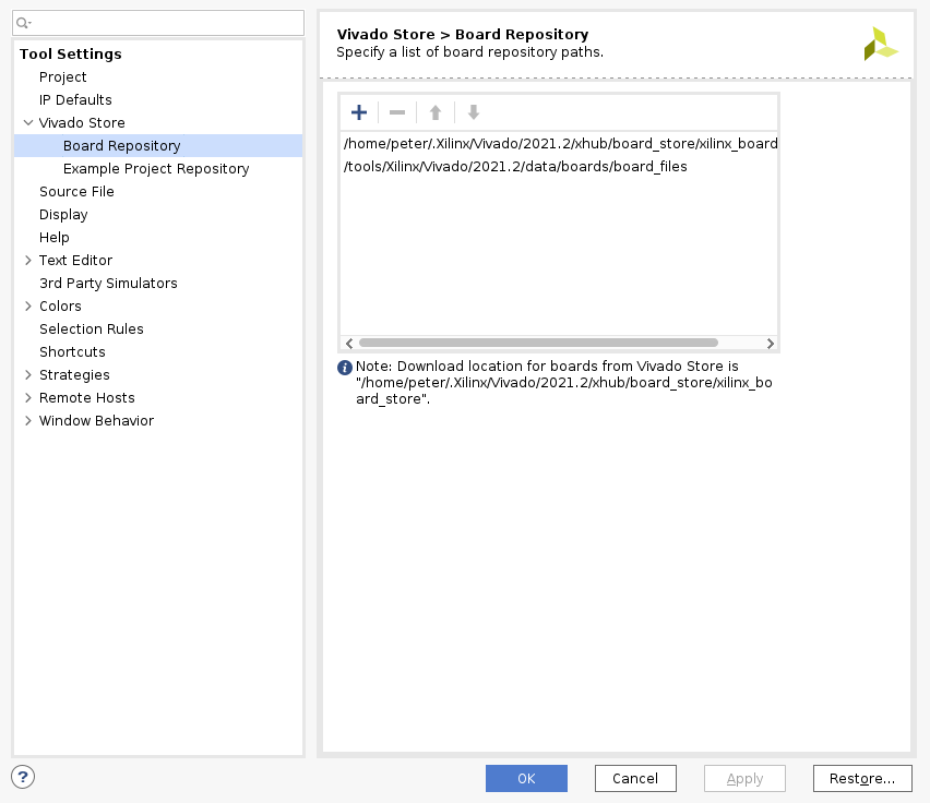
First, create a new RTL project named tensil-pynqz1 and add Verilog files generated by the Tensil RTL tool.

Choose boards and search for PYNQ. Select PYNQ-Z1 with file version 1.0.
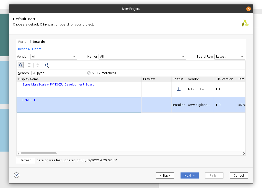
Under IP INTEGRATOR, click Create Block Design.
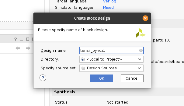
Drag top_pynqz1 from the Sources tab onto the block design diagram. You should see the Tensil RTL block with its interfaces.
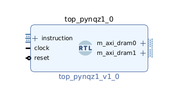
Next, click the plus + button in the Block Diagram toolbar (upper left) and select “ZYNQ7 Processing System” (you may need to use the search box). Do the same for “Processor System Reset”. The Zynq block represents the “hard” part of the Xilinx platform, which includes ARM processors, DDR interfaces, and much more. The Processor System Reset is a utility box that provides the design with correctly synchronized reset signals.
Click “Run Block Automation” and “Run Connection Automation”. Check “All Automation”.
Double-click ZYNQ7 Processing System. First, go to Clock Configuration and ensure PL Fabric Clocks have FCLK_CLK0 checked and set to 50MHz.
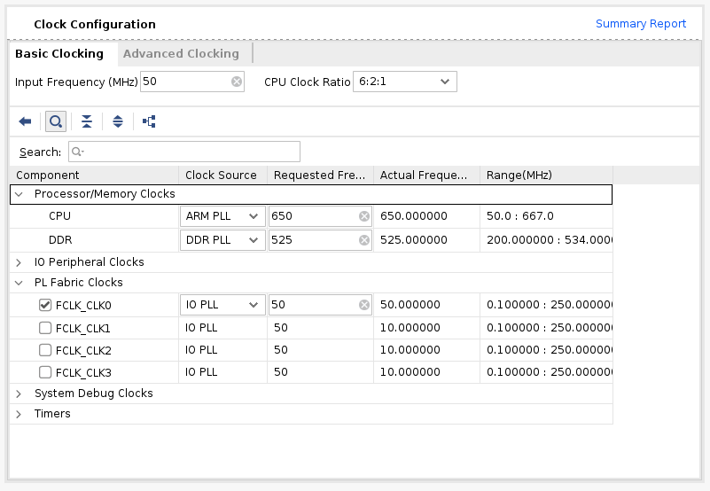
Then, go to PS-PL Configuration. Check S AXI HP0 FPD, S AXI HP1 FPD, and S AXI HP2 FPD. These changes will configure all the necessary interfaces between Processing System (PS) and Programmable Logic (PL) necessary for our design.
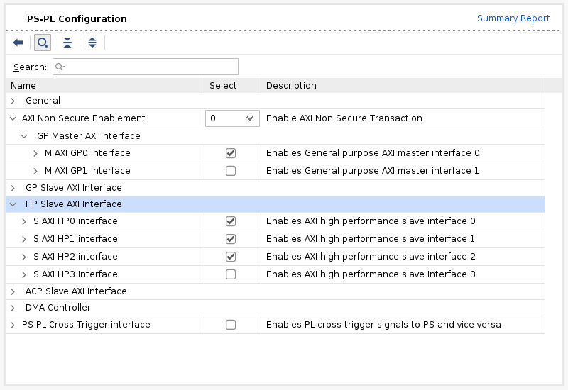
Again, click the plus + button in the Block Diagram toolbar and select “AXI SmartConnect”. We’ll need 4 instances of SmartConnect. First 3 instances (smartconnect_0 to smartconnect_2) are necessary to convert AXI version 4 interfaces of the TCU and the instruction DMA block to AXI version 3 on the PS. The smartconnect_3 is necessary to expose DMA control registers to the Zynq CPU, which will enable software to control the DMA transactions. Double-click each one and set “Number of Slave and Master Interfaces” to 1.
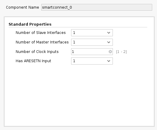
Now, connect m_axi_dram0 and m_axi_dram1 ports on Tensil block to S00_AXI on smartconnect_0 and smartconnect_1 correspondigly. Then connect SmartConnect M00_AXI ports to S_AXI_HP0 and S_AXI_HP2 on Zynq block correspondingly. The TCU has two DRAM banks to enable their parallel operation by utilizing PS ports with dedicated connectivity to the memory.
Next, click the plus + button in the Block Diagram toolbar and select “AXI Direct Memory Access” (DMA). The DMA block is used to organize the feeding of the Tensil program to the TCU without keeping the PS ARM processor busy.
Double-click it. Disable “Scatter Gather Engine” and “Write Channel”. Change “Width of Buffer Length Register” to be 26 bits. Select “Memory Map Data Width” and “Stream Data Width” to be 64 bits. Change “Max Burst Size” to 256.

Connect the instruction port on the Tensil top block to the M_AXIS_MM2S on the AXI DMA block. Then, connect M_AXI_MM2S on the AXI DMA block to S00_AXI on smartconnect_2 and, finally, connect smartconnect_2 M00_AXI port to S_AXI_HP1 on Zynq.
Connect M00_AXI on smartconnect_3 to S_AXI_LITE on the AXI DMA block. Connect S00_AXI on the AXI SmartConnect to M_AXI_GP0 on the Zynq block.
Finally, click “Run Connection Automation” and check “All Automation”. By doing this, we connect all the clocks and resets. Click the “Regenerate Layout” button in the Block Diagram toolbar to make the diagram look nice.
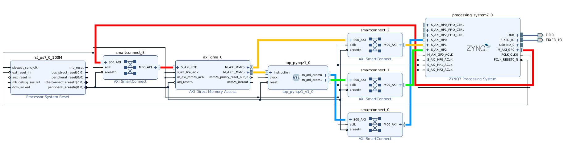
Next, switch to the “Address Editor” tab. Click the “Assign All” button in the toolbar. By doing this, we assign address spaces to various AXI interfaces. For example, the instruction DMA (axi_dma_0) and Tensil (m_axi_dram0 and m_axi_dram1) gain access to the entire address space on the PYNQ Z1 board. The PS gains access to the control registers for the instruction DMA.
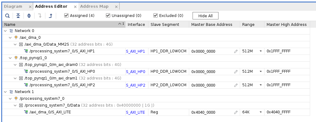
Back in the Block Diagram tab, click the “Validate Design” (or F6) button. You should see the message informing you of successful validation! You can now close the Block Design by clicking x in the right upper corner.
The final step is to create the HDL wrapper for our design, which will tie everything together and enable synthesis and implementation. Right-click the tensil_pynqz1 item in the Sources tab and choose “Create HDL Wrapper”. Keep “Let Vivado manage wrapper and auto-update” selected. Wait for the Sources tree to be fully updated and right-click on tensil_pynqz1_wrapper. Choose Set as Top.
Now it’s time to let Vivado perform synthesis and implementation and write the resulting bitstream. In the Flow Navigator sidebar, click on “Generate Bitstream” and hit OK. Vivado will start synthesizing our Tensil design – this may take around 15 minutes. When done, you can observe some vital stats in the Project Summary. First, look at utilization, which shows what percentage of each FPGA resource our design is using. Note how we kept BRAM and DSP utilization reasonably low.
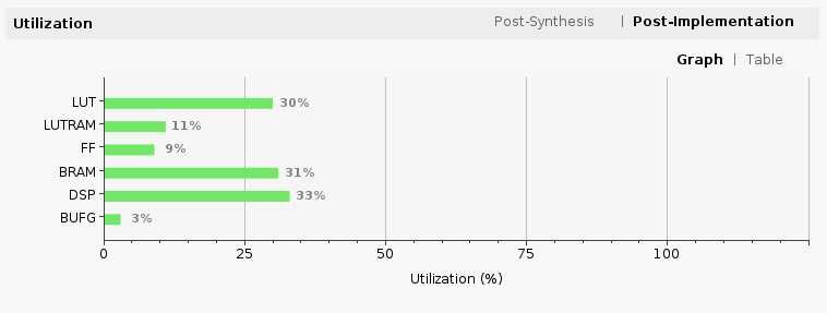
The second is timing, which tells us about how long it takes for signals to propagate in our programmable logic (PL). The “Worst Negative Slack” being a positive number is good news – our design meets propagation constraints for all nets at the specified clock speed!
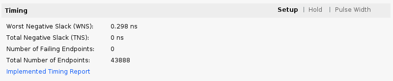
5. Compile ML model for TCU
The second branch of the Tensil toolchain flow is to compile the ML model to a Tensil binary consisting of TCU instructions, which are executed by the TCU hardware directly. For this tutorial, we will use ResNet20 trained on the CIFAR dataset. The model is included in the Tensil docker image at /demo/models/resnet20v2_cifar.onnx. From within the Tensil docker container, run the following command.
tensil compile -a /demo/arch/pynqz1.tarch -m /demo/models/resnet20v2_cifar.onnx -o "Identity:0" -s true
We’re using the ONNX version of the model, but the Tensil compiler also supports TensorFlow, which you can try by compiling the same model in TensorFlow frozen graph form at /demo/models/resnet20v2_cifar.pb.
tensil compile -a /demo/arch/pynqz1.tarch -m /demo/models/resnet20v2_cifar.pb -o "Identity" -s true
The resulting compiled files are listed in the ARTIFACTS table. The manifest (tmodel) is a plain text JSON description of the compiled model. The Tensil program (tprog) and weights data (tdata) are both binaries to be used by the TCU during execution. The Tensil compiler also prints a COMPILER SUMMARY table with interesting stats for both the TCU architecture and the model.
------------------------------------------------------------------------------------------
COMPILER SUMMARY
------------------------------------------------------------------------------------------
Model:                                           resnet20v2_cifar_onnx_pynqz1
Data type:                                       FP16BP8
Array size:                                      8
Consts memory size (vectors/scalars/bits):       1,048,576                    8,388,608 20
Vars memory size (vectors/scalars/bits):         1,048,576                    8,388,608 20
Local memory size (vectors/scalars/bits):        8,192                        65,536    13
Accumulator memory size (vectors/scalars/bits):  2,048                        16,384    11
Stride #0 size (bits):                           3
Stride #1 size (bits):                           3
Operand #0 size (bits):                          16
Operand #1 size (bits):                          24
Operand #2 size (bits):                          16
Instruction size (bytes):                        8
Consts memory maximum usage (vectors/scalars):   71,341                       570,728
Vars memory maximum usage (vectors/scalars):     26,624                       212,992
Consts memory aggregate usage (vectors/scalars): 71,341                       570,728
Vars memory aggregate usage (vectors/scalars):   91,170                       729,360
Number of layers:                                23
Total number of instructions:                    258,037
Compilation time (seconds):                      25.487
True consts scalar size:                         568,466
Consts utilization (%):                          97.545
True MACs (M):                                   61.476
MAC efficiency (%):                              0.000
------------------------------------------------------------------------------------------
6. Execute using PYNQ
Now it’s time to put everything together on our development board. For this, we first need to set up the PYNQ environment. This process starts with downloading the SD card image for our development board. There’s the detailed instruction for setting board connectivity on the PYNQ documentation website. You should be able to open Jupyter notebooks and run some examples.
Now that PYNQ is up and running, the next step is to scp the Tensil driver for PYNQ. Start by cloning the Tensil GitHub repository to your work station and then copy drivers/tcu_pynq to /home/xilinx/tcu_pynq onto your board.
git clone [email protected]:tensil-ai/tensil.git
scp -r tensil/drivers/tcu_pynq [email protected]:
We also need to scp the bitstream and compiler artifacts.
Next we’ll copy over the bitstream, which contains the FPGA configuration resulting from Vivado synthesis and implementation. PYNQ also needs a hardware handoff file that describes FPGA components accessible to the host, such as DMA. Place both files in /home/xilinx on the development board. Assuming you are in the Vivado project directory, run the following commands to copy files over.
scp tensil-pynqz1.runs/impl_1/tensil_pynqz1_wrapper.bit [email protected]:tensil_pynqz1.bit
scp tensil-pynqz1.gen/sources_1/bd/tensil_pynqz1/hw_handoff/tensil_pynqz1.hwh [email protected]:
Note that we renamed bitstream to match the hardware handoff file name.
Now, copy the .tmodel, .tprog and .tdata artifacts produced by the compiler to /home/xilinx on the board.
scp resnet20v2_cifar_onnx_pynqz1.t* [email protected]:
The last thing needed to run our ResNet model is the CIFAR dataset. You can get it from Kaggle or run the commands below (since we only need the test batch, we remove the training batches to reduce the file size). Put these files in /home/xilinx/cifar-10-batches-py/ on your development board.
wget http://www.cs.toronto.edu/~kriz/cifar-10-python.tar.gz
tar xfvz cifar-10-python.tar.gz
rm cifar-10-batches-py/data_batch_*
scp -r cifar-10-batches-py [email protected]:
We are finally ready to fire up the PYNQ Jupyter notebook and run the ResNet model on TCU.
Jupyter notebook
First, we import the Tensil PYNQ driver and other required utilities.
import sys
sys.path.append('/home/xilinx')

# Needed to run inference on TCU
import time
import numpy as np
import pynq
from pynq import Overlay
from tcu_pynq.driver import Driver
from tcu_pynq.architecture import pynqz1

# Needed for unpacking and displaying image data
%matplotlib inline
import matplotlib.pyplot as plt
import pickle
Now, initialize the PYNQ overlay from the bitstream and instantiate the Tensil driver using the TCU architecture and the overlay’s DMA configuration. Note that we are passing axi_dma_0 object from the overlay – the name matches the DMA block in the Vivado design.
overlay = Overlay('/home/xilinx/tensil_pynqz1.bit')
tcu = Driver(pynqz1, overlay.axi_dma_0)
The Tensil PYNQ driver includes the PYNQ Z1 architecture definition. Here it is in an excerpt from architecture.py: you can see that it matches the architecture we used previously.
pynqz1 = Architecture(
    data_type=DataType.FP16BP8,
    array_size=8,
    dram0_depth=1048576,
    dram1_depth=1048576,
    local_depth=8192,
    accumulator_depth=2048,
    simd_registers_depth=1,
    stride0_depth=8,
    stride1_depth=8,
)
Next, let’s load CIFAR images from the test_batch.
def unpickle(file):
    with open(file, 'rb') as fo:
        d = pickle.load(fo, encoding='bytes')
    return d

cifar = unpickle('/home/xilinx/cifar-10-batches-py/test_batch')
data = cifar[b'data']
labels = cifar[b'labels']

data = data[10:20]
labels = labels[10:20]

data_norm = data.astype('float32') / 255
data_mean = np.mean(data_norm, axis=0)
data_norm -= data_mean

cifar_meta = unpickle('/home/xilinx/cifar-10-batches-py/batches.meta')
label_names = [b.decode() for b in cifar_meta[b'label_names']]

def show_img(data, n):
    plt.imshow(np.transpose(data[n].reshape((3, 32, 32)), axes=[1, 2, 0]))

def get_img(data, n):
    img = np.transpose(data_norm[n].reshape((3, 32, 32)), axes=[1, 2, 0])
    img = np.pad(img, [(0, 0), (0, 0), (0, tcu.arch.array_size - 3)], 'constant', constant_values=0)
    return img.reshape((-1, tcu.arch.array_size))

def get_label(labels, label_names, n):
    label_idx = labels[n]
    name = label_names[label_idx]
    return (label_idx, name)
To test, extract one of the images.
n = 7
img = get_img(data, n)
label_idx, label = get_label(labels, label_names, n)
show_img(data, n)
You should see the image.
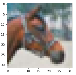
Next, load the tmodel manifest for the model into the driver. The manifest tells the driver where to find the other two binary files (program and weights data).
tcu.load_model('/home/xilinx/resnet20v2_cifar_onnx_pynqz1.tmodel')
Finally, run the model and print the results! The call to tcu.run(inputs) is where the magic happens. We’ll convert the ResNet classification result vector into CIFAR labels. Note that if you are using the ONNX model, the input and output are named x:0 and Identity:0 respectively. For the TensorFlow model they are named x and Identity.
inputs = {'x:0': img}

start = time.time()
outputs = tcu.run(inputs)
end = time.time()
print("Ran inference in {:.4}s".format(end - start))
print()

classes = outputs['Identity:0'][:10]
result_idx = np.argmax(classes)
result = label_names[result_idx]
print("Output activations:")
print(classes)
print()
print("Result: {} (idx = {})".format(result, result_idx))
print("Actual: {} (idx = {})".format(label, label_idx))
Here is the expected result:
Ran inference in 0.1513s

Output activations:
[-19.49609375 -12.37890625  -8.01953125  -6.01953125  -6.609375
  -4.921875    -7.71875      2.0859375   -9.640625    -7.85546875]

Result: horse (idx = 7)
Actual: horse (idx = 7)
Congratulations! You ran a machine learning model a custom ML accelerator that you built on your own work station! Just imagine the things you could do with it…
Wrap-up
In this tutorial we used Tensil to show how to run machine learning (ML) models on FPGA. We went through a number of steps to get here, including installing Tensil, choosing an architecture, generating an RTL design, synthesizing the desing, compiling the ML model and finally executing the model using PYNQ.
If you made it all the way through, big congrats! You’re ready to take things to the next level by trying out your own model and architecture. Join us on Discord to say hello and ask questions, or send an email to [email protected].
6 - Learn Tensil with ResNet and Ultra96
Originally posted here.
Introduction
This tutorial will use the Avnet Ultra96 V2 development board and Tensil’s open-source inference accelerator to show how to run machine learning (ML) models on FPGA. We will be using ResNet-20 trained on the CIFAR dataset. These steps should work for any supported ML model – currently all the common state-of-the-art convolutional neural networks are supported. Try it with your model!
We’ll give detailed end-to-end coverage that is easy to follow. In addition, we include in-depth explanations to get a good understanding of the technology behind it all, including the Tensil and Xilinx Vivado toolchains and PYNQ framework.
If you get stuck or find an error, you can ask a question on our Discord or send an email to [email protected].
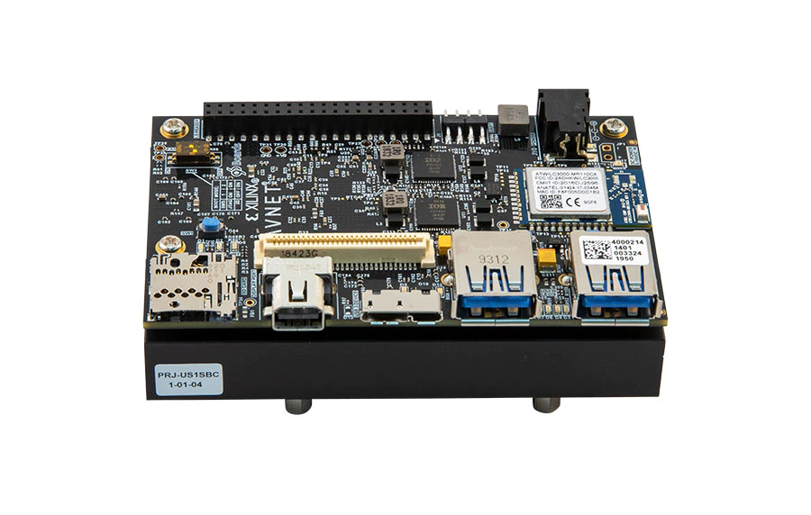
Overview
Before we start, let’s look at the Tensil toolchain flow to get a bird’s eye view of what we want to accomplish. We’ll follow these steps:
- Get Tensil
- Choose architecture
- Generate TCU accelerator design (RTL code)
- Synthesize for Ultra96
- Compile ML model for TCU
- Execute using PYNQ

1. Get Tensil
First, we need to get the Tensil toolchain. The easiest way is to pull the Tensil docker container from Docker Hub. The following command will pull the image and then run the container.
docker pull tensilai/tensil
docker run -v $(pwd):/work -w /work -it tensilai/tensil bash
2. Choose architecture
Tensil’s strength is customizability, making it suitable for a very wide range of applications. The Tensil architecture definition file (.tarch) specifies the parameters of the architecture to be implemented. These parameters are what make Tensil flexible enough to work for small embedded FPGAs as well as large data-center FPGAs. Our example will select parameters that provide the highest utilization of resources on the ZU3EG FPGA part at the core of the Ultra96 board. The container image conveniently includes the architecture file for the Ultra96 development board at /demo/arch/ultra96v2.tarch. Let’s take a look at what’s inside.
{
    "data_type": "FP16BP8",
    "array_size": 16,
    "dram0_depth": 2097152,
    "dram1_depth": 2097152,
    "local_depth": 20480,
    "accumulator_depth": 4096,
    "simd_registers_depth": 1,
    "stride0_depth": 8,
    "stride1_depth": 8
}
The file contains a JSON object with several parameters. The first, data_type, defines the data type used throughout the Tensor Compute Unit (TCU), including in the systolic array, SIMD ALUs, accumulators, and local memory. We will use 16-bit fixed-point with an 8-bit base point (FP16BP8), which in most cases allows simple rounding of 32-bit floating-point models without the need for quantization. Next, array_size defines a systolic array size of 16x16, which results in 256 parallel multiply-accumulate (MAC) units. This number was chosen to maximize the utilization of DSP units available on ZU3EG, but if you needed to use some DSPs for another application in parallel, you could decrease it to free some up.
With dram0_depth and dram1_depth, we define the size of DRAM0 and DRAM1 memory buffers on the host side. These buffers feed the TCU with the model’s weights and inputs, and also store intermediate results and outputs. Note that these memory sizes are in number of vectors, which means array size (16) multiplied by data type size (16-bits) for a total of 256 bits per vector.
Next, we define the size of the local and accumulator memories which will be implemented on the FPGA fabric itself. The difference between the accumulators and the local memory is that accumulators can perform a write-accumulate operation in which the input is added to the data already stored, as opposed to simply overwriting it. The total size of accumulators plus local memory is again selected to maximize the utilization of BRAM resources on ZU3EG, but if necessary you could reduce these to free up resources needed elsewhere.
With simd_registers_depth, we specify the number of registers included in each SIMD ALU, which can perform SIMD operations on stored vectors used for ML operations like ReLU activation. Increasing this number is only needed rarely, to help compute special activation functions. Finally, stride0_depth and stride1_depth specify the number of bits to use for enabling “strided” memory reads and writes. It’s unlikely you’ll ever need to change this parameter.
3. Generate TCU accelerator design (RTL code)
Now that we’ve selected our architecture, it’s time to run the Tensil RTL generator. RTL stands for “Register Transfer Level” – it’s a type of code that specifies digital logic stuff like wires, registers and low-level logic. Special tools like Xilinx Vivado or yosys can synthesize RTL for FPGAs and even ASICs.
To generate a design using our chosen architecture, run the following command inside the Tensil toolchain docker container:
tensil rtl -a /demo/arch/ultra96v2.tarch -s true -d 128
Note the -d 128 parameter, which specifies that the generated RTL will be compatible with 128-bit AXI interfaces supported by the ZU3EG part. This command will produce several Verilog files listed in the ARTIFACTS table printed out at the end. It also prints the RTL SUMMARY table with some of the essential parameters of the resulting RTL.
-----------------------------------------------------------------------
RTL SUMMARY
-----------------------------------------------------------------------
Data type:                                      FP16BP8
Array size:                                     16
Consts memory size (vectors/scalars/bits):      2,097,152 33,554,432 21
Vars memory size (vectors/scalars/bits):        2,097,152 33,554,432 21
Local memory size (vectors/scalars/bits):       20,480    327,680    15
Accumulator memory size (vectors/scalars/bits): 4,096     65,536     12
Stride #0 size (bits):                          3
Stride #1 size (bits):                          3
Operand #0 size (bits):                         24
Operand #1 size (bits):                         24
Operand #2 size (bits):                         16
Instruction size (bytes):                       9
-----------------------------------------------------------------------
4. Synthesize for Ultra96
It is now time to start Xilinx Vivado. I will be using version 2021.2, which you can download free of charge (for prototyping) at the Xilinx website.
First, create a new RTL project named tensil-ultra96v2 and add Verilog files generated by the Tensil RTL tool.
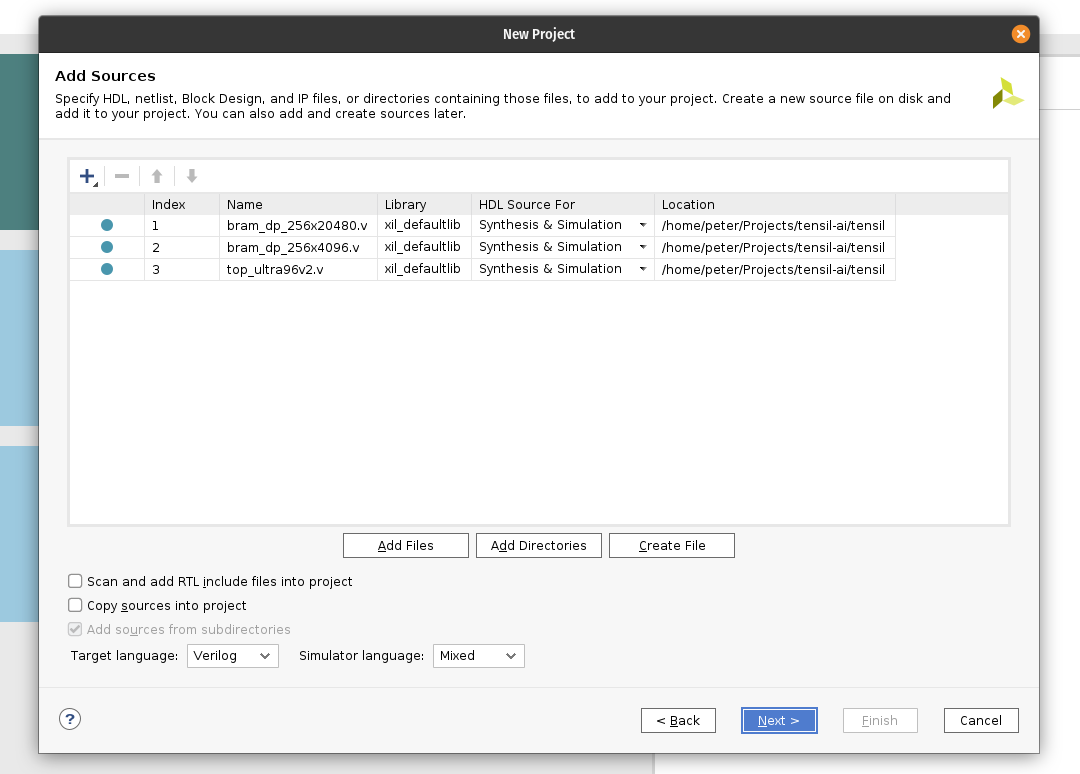
Choose boards and search for Ultra96. Select Ultra96-V2 Single Board Computer with file version 1.2. You may need to click the Install icon in the Status column. (If you don’t find the board, click on the Refresh button below.)

Under IP INTEGRATOR, click Create Block Design.
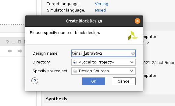
Drag top_ultra96v2 from the Sources tab onto the block design diagram. You should see the Tensil RTL block with its interfaces.
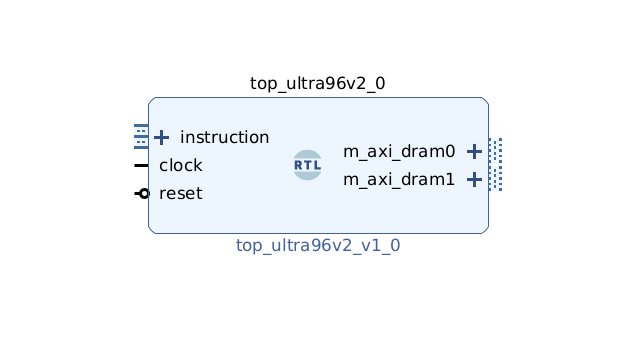
Next, click the plus + button in the Block Diagram toolbar (upper left) and select “Zynq UltraScale+ MPSoC” (you may need to use the search box). Do the same for “Processor System Reset”. The Zynq block represents the “hard” part of the Xilinx platform, which includes ARM processors, DDR interfaces, and much more. The Processor System Reset is a utility box that provides the design with correctly synchronized reset signals.
Click “Run Block Automation” and “Run Connection Automation”. Check “All Automation”.
Double-click Zynq UltraScale+ MPSoC. First, go to Clock Configuration and ensure PL Fabric Clocks have PL0 checked and set to 100MHz.
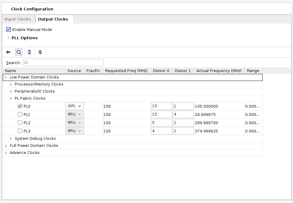
Then, go to PS-PL Configuration. Uncheck AXI HPM1 FPD and check AXI HP1 FPD, AXI HP2 FPD, and AXI HP3 FPD. These changes will configure all the necessary interfaces between Processing System (PS) and Programmable Logic (PL) necessary for our design.
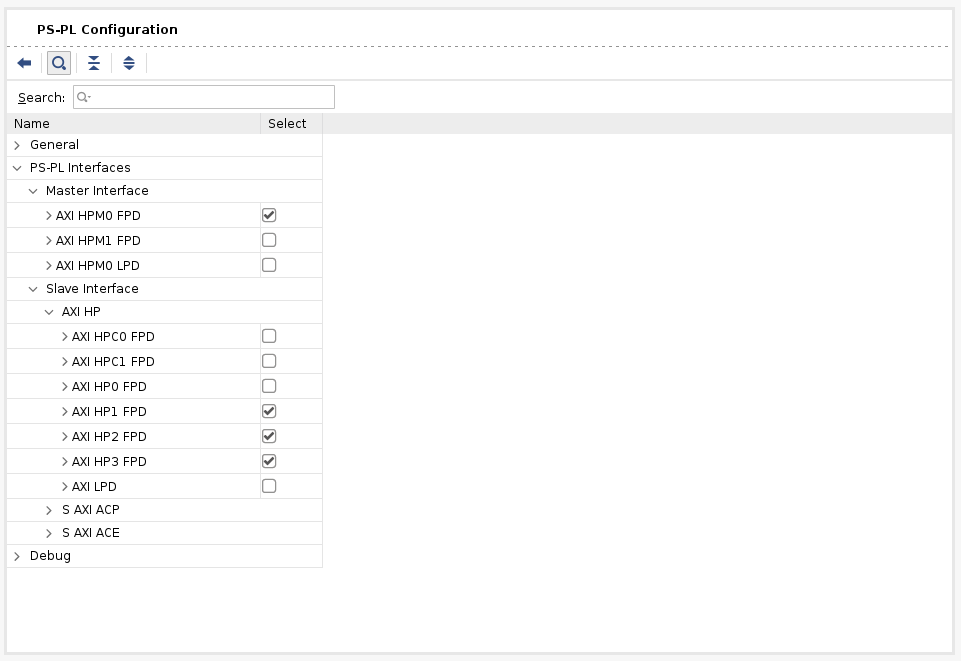
Now, connect m_axi_dram0 and m_axi_dram1 ports on Tensil block to S_AXI_HP1_FPD and S_AXI_HP2_FPD on Zynq block correspondingly. The TCU has two DRAM banks to enable their parallel operation by utilizing separate PS ports.
Next, click the plus + button in the Block Diagram toolbar and select “AXI Direct Memory Access” (DMA). The DMA block is used to organize the feeding of the Tensil program to the TCU without keeping the PS ARM processor busy.
Double-click it. Disable “Scatter Gather Engine” and “Write Channel”. Change “Width of Buffer Length Register” to be 26 bits. Select “Memory Map Data Width” and “Stream Data Width” to be 128 bits. Change “Max Burst Size” to 256.
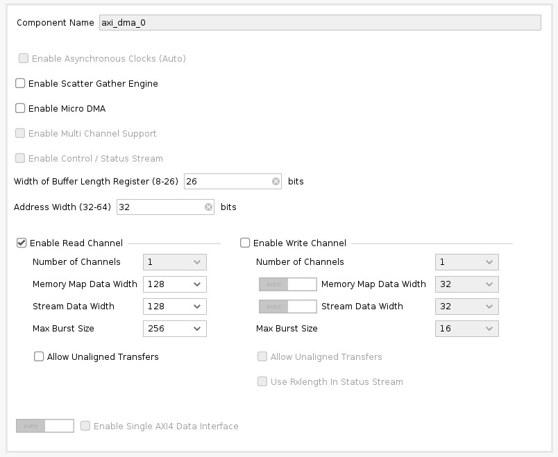
Connect the instruction port on the Tensil top block to M_AXIS_MM2S on the AXI DMA block. Then, connect M_AXI_MM2S on the AXI DMA block to S_AXI_HP3_FPD on Zynq.
Once again, click the plus + button in the Block Diagram toolbar and select “AXI SmartConnect”. The SmartConnect is necessary to expose DMA control registers to the Zynq CPU, which will enable software to control the DMA transactions. Double-click it and set “Number of Slave and Master Interfaces” to 1.
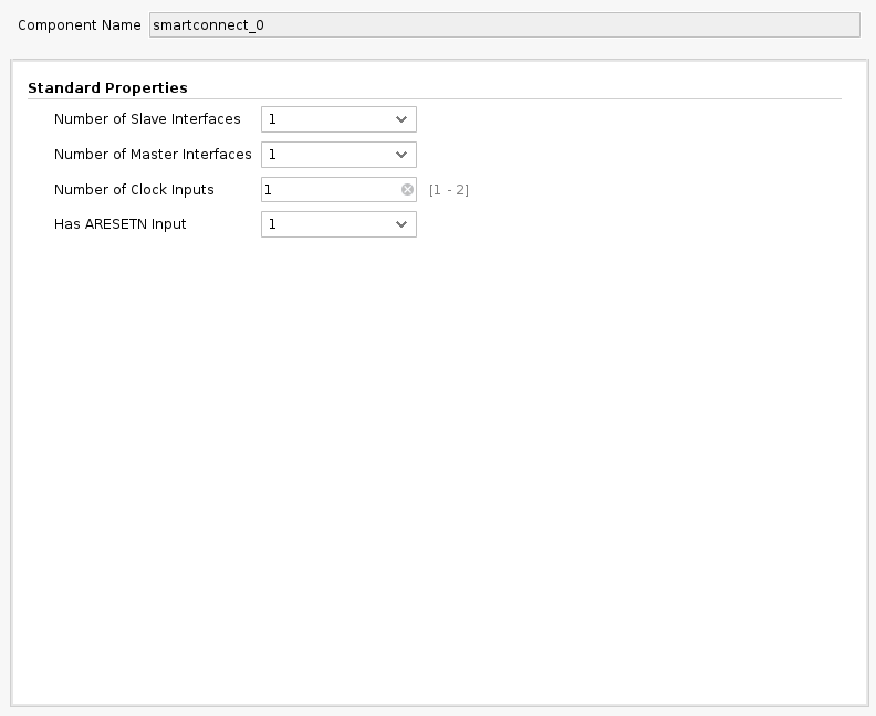
Connect M00_AXI on the AXI SmartConnect block to S_AXI_LITE on the AXI DMA block. Connect S00_AXI on the AXI SmartConnect to M_AXI_HPM0_FPD on the Zynq block.
Finally, click “Run Connection Automation” and check “All Automation”. By doing this, we connect all the clocks and resets. Click the “Regenerate Layout” button in the Block Diagram toolbar to make the diagram look nice.
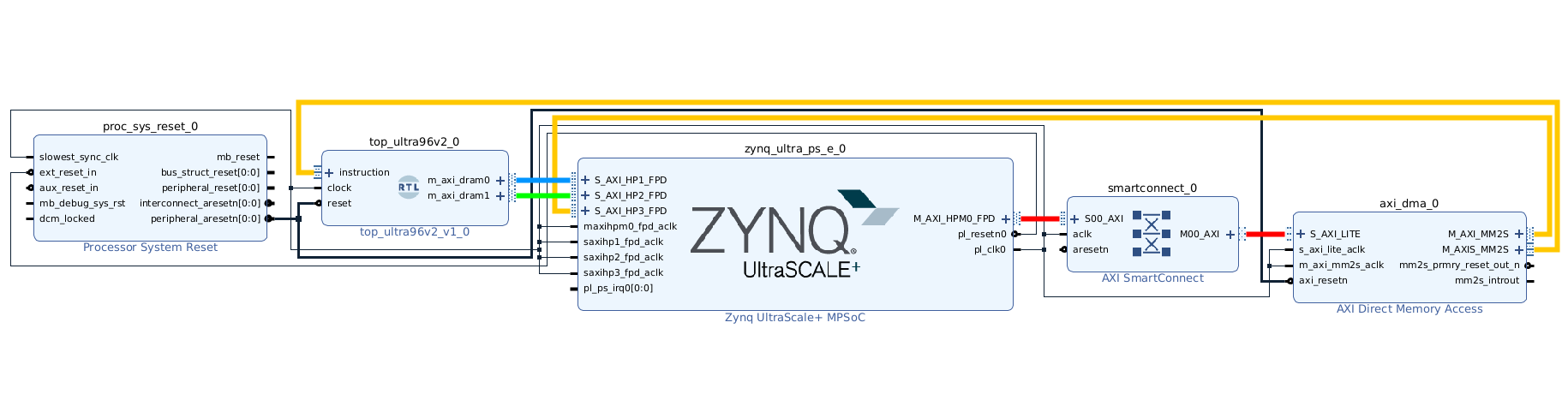
Next, switch to the “Address Editor” tab. Click the “Assign All” button in the toolbar. By doing this, we assign address spaces to various AXI interfaces. For example, m_axi_dram0 and m_axi_dram1 gain access to the entire address space on the Ultra96 board, including DDR memory and control register spaces. We only need access to DDR, so you can manually exclude the register address space if you know what you’re doing.
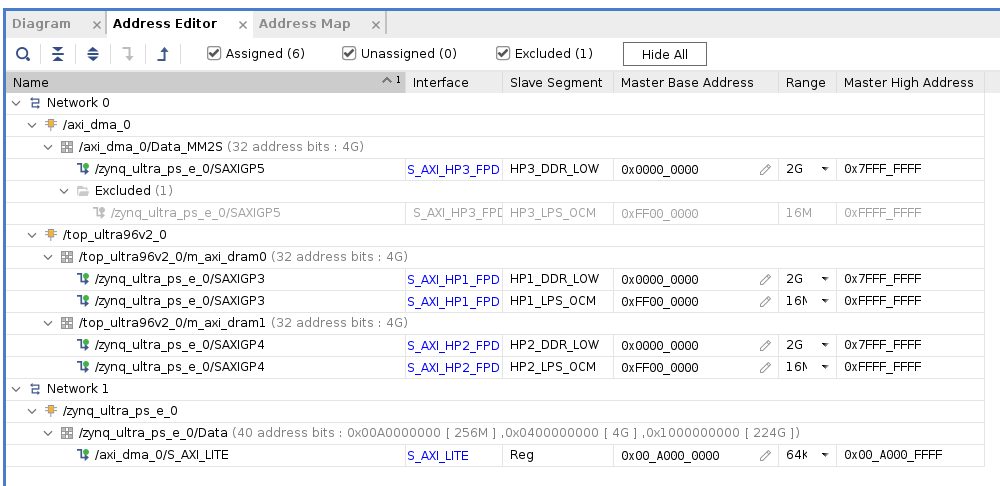
Back in the Block Diagram tab, click the “Validate Design” (or F6) button. You should see the message informing you of successful validation! You can now close the Block Design by clicking x in the right upper corner.
The final step is to create the HDL wrapper for our design, which will tie everything together and enable synthesis and implementation. Right-click the tensil_ultra96v2 item in the Sources tab and choose “Create HDL Wrapper”. Keep “Let Vivado manage wrapper and auto-update” selected. Wait for the Sources tree to be fully updated and right-click on tensil_ultra96v2_wrapper. Choose Set as Top.
Now it’s time to let Vivado perform synthesis and implementation and write the resulting bitstream. In the Flow Navigator sidebar, click on “Generate Bitstream” and hit OK. Vivado will start synthesizing our Tensil design – this may take around 15 minutes. When done, you can observe some vital stats in the Project Summary. First, look at utilization, which shows what percentage of each FPGA resource our design is using. Note how we pushed BRAM and DSP resources to high utilization.
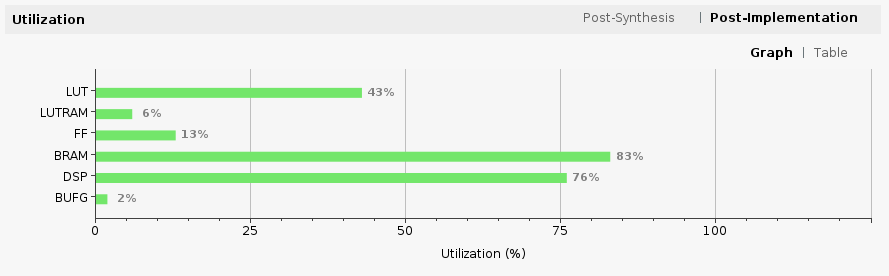
The second is timing, which tells us about how long it takes for signals to propagate in our programmable logic (PL). The “Worst Negative Slack” being a positive number is good news – our design meets propagation constraints for all nets at the specified clock speed!
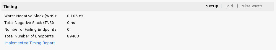
5. Compile ML model for TCU
The second branch of the Tensil toolchain flow is to compile the ML model to a Tensil binary consisting of TCU instructions, which are executed by the TCU hardware directly. For this tutorial, we will use ResNet20 trained on the CIFAR dataset. The model is included in the Tensil docker image at /demo/models/resnet20v2_cifar.onnx. From within the Tensil docker container, run the following command.
tensil compile -a /demo/arch/ultra96v2.tarch -m /demo/models/resnet20v2_cifar.onnx -o "Identity:0" -s true
We’re using the ONNX version of the model, but the Tensil compiler also supports TensorFlow, which you can try by compiling the same model in TensorFlow frozen graph form at /demo/models/resnet20v2_cifar.pb.
tensil compile -a /demo/arch/ultra96v2.tarch -m /demo/models/resnet20v2_cifar.pb -o "Identity" -s true
The resulting compiled files are listed in the ARTIFACTS table. The manifest (tmodel) is a plain text JSON description of the compiled model. The Tensil program (tprog) and weights data (tdata) are both binaries to be used by the TCU during execution. The Tensil compiler also prints a COMPILER SUMMARY table with interesting stats for both the TCU architecture and the model.
----------------------------------------------------------------------------------------------
COMPILER SUMMARY
----------------------------------------------------------------------------------------------
Model:                                           resnet20v2_cifar_onnx_ultra96v2
Data type:                                       FP16BP8
Array size:                                      16
Consts memory size (vectors/scalars/bits):       2,097,152                       33,554,432 21
Vars memory size (vectors/scalars/bits):         2,097,152                       33,554,432 21
Local memory size (vectors/scalars/bits):        20,480                          327,680    15
Accumulator memory size (vectors/scalars/bits):  4,096                           65,536     12
Stride #0 size (bits):                           3
Stride #1 size (bits):                           3
Operand #0 size (bits):                          24
Operand #1 size (bits):                          24
Operand #2 size (bits):                          16
Instruction size (bytes):                        9
Consts memory maximum usage (vectors/scalars):   35,743                          571,888
Vars memory maximum usage (vectors/scalars):     13,312                          212,992
Consts memory aggregate usage (vectors/scalars): 35,743                          571,888
Vars memory aggregate usage (vectors/scalars):   46,097                          737,552
Number of layers:                                23
Total number of instructions:                    102,741
Compilation time (seconds):                      30.066
True consts scalar size:                         568,474
Consts utilization (%):                          97.210
True MACs (M):                                   61.476
MAC efficiency (%):                              0.000
----------------------------------------------------------------------------------------------
6. Execute using PYNQ
Now it’s time to put everything together on our development board. For this, we first need to set up the PYNQ environment. This process starts with downloading the SD card image for our development board. There’s the detailed instruction for setting board connectivity on the PYNQ documentation website. You should be able to open Jupyter notebooks and run some examples.
There is one caveat that needs addressing once PYNQ is installed. On the default PYNQ image, the setting for the Linux kernel CMA (Contiguous Memory Allocator) area size is 128MB. Given our Tensil architecture, the default CMA size is too small. To address this, you’ll need to download our patched kernel, copy it to /boot, and reboot your board. Note that the patched kernel is built for PYNQ 2.7 and will not work with other versions. To patch the kernel, run these commands:
wget https://s3.us-west-1.amazonaws.com/downloads.tensil.ai/pynq/2.7/ultra96v2/image.ub
scp image.ub [email protected]:
ssh [email protected]
sudo cp /boot/image.ub /boot/image.ub.backup
sudo cp image.ub /boot/
rm image.ub
sudo reboot
Now that PYNQ is up and running, the next step is to scp the Tensil driver for PYNQ. Start by cloning the Tensil GitHub repository to your work station and then copy drivers/tcu_pynq to /home/xilinx/tcu_pynq onto your board.
git clone [email protected]:tensil-ai/tensil.git
scp -r tensil/drivers/tcu_pynq [email protected]:
We also need to scp the bitstream and compiler artifacts.
Next we’ll copy over the bitstream, which contains the FPGA configuration resulting from Vivado synthesis and implementation. PYNQ also needs a hardware handoff file that describes FPGA components accessible to the host, such as DMA. Place both files in /home/xilinx on the development board. Assuming you are in the Vivado project directory, run the following commands to copy files over.
scp tensil-ultra96v2.runs/impl_1/tensil_ultra96v2_wrapper.bit [email protected]:tensil_ultra96v2.bit
scp tensil-ultra96v2.gen/sources_1/bd/tensil_ultra96v2/hw_handoff/tensil_ultra96v2.hwh [email protected]:
Note that we renamed bitstream to match the hardware handoff file name.
Now, copy the .tmodel, .tprog and .tdata artifacts produced by the compiler to /home/xilinx on the board.
scp resnet20v2_cifar_onnx_ultra96v2.t* [email protected]:
The last thing needed to run our ResNet model is the CIFAR dataset. You can get it from Kaggle or run the commands below (since we only need the test batch, we remove the training batches to reduce the file size). Put these files in /home/xilinx/cifar-10-batches-py/ on your development board.
wget http://www.cs.toronto.edu/~kriz/cifar-10-python.tar.gz
tar xfvz cifar-10-python.tar.gz
rm cifar-10-batches-py/data_batch_*
scp -r cifar-10-batches-py [email protected]:
We are finally ready to fire up the PYNQ Jupyter notebook and run the ResNet model on TCU.
Jupyter notebook
First, we import the Tensil PYNQ driver and other required utilities.
import sys
sys.path.append('/home/xilinx')

# Needed to run inference on TCU
import time
import numpy as np
import pynq
from pynq import Overlay
from tcu_pynq.driver import Driver
from tcu_pynq.architecture import ultra96

# Needed for unpacking and displaying image data
%matplotlib inline
import matplotlib.pyplot as plt
import pickle
Now, initialize the PYNQ overlay from the bitstream and instantiate the Tensil driver using the TCU architecture and the overlay’s DMA configuration. Note that we are passing axi_dma_0 object from the overlay – the name matches the DMA block in the Vivado design.
overlay = Overlay('/home/xilinx/tensil_ultra96v2.bit')
tcu = Driver(ultra96, overlay.axi_dma_0)
The Tensil PYNQ driver includes the Ultra96 architecture definition. Here it is in an excerpt from architecture.py: you can see that it matches the architecture we used previously.
ultra96 = Architecture(
    data_type=DataType.FP16BP8,
    array_size=16,
    dram0_depth=2097152,
    dram1_depth=2097152,
    local_depth=20480,
    accumulator_depth=4096,
    simd_registers_depth=1,
    stride0_depth=8,
    stride1_depth=8,
)
Next, let’s load CIFAR images from the test_batch.
def unpickle(file):
    with open(file, 'rb') as fo:
        d = pickle.load(fo, encoding='bytes')
    return d

cifar = unpickle('/home/xilinx/cifar-10-batches-py/test_batch')
data = cifar[b'data']
labels = cifar[b'labels']

data = data[10:20]
labels = labels[10:20]

data_norm = data.astype('float32') / 255
data_mean = np.mean(data_norm, axis=0)
data_norm -= data_mean

cifar_meta = unpickle('/home/xilinx/cifar-10-batches-py/batches.meta')
label_names = [b.decode() for b in cifar_meta[b'label_names']]

def show_img(data, n):
    plt.imshow(np.transpose(data[n].reshape((3, 32, 32)), axes=[1, 2, 0]))

def get_img(data, n):
    img = np.transpose(data_norm[n].reshape((3, 32, 32)), axes=[1, 2, 0])
    img = np.pad(img, [(0, 0), (0, 0), (0, tcu.arch.array_size - 3)], 'constant', constant_values=0)
    return img.reshape((-1, tcu.arch.array_size))

def get_label(labels, label_names, n):
    label_idx = labels[n]
    name = label_names[label_idx]
    return (label_idx, name)
To test, extract one of the images.
n = 9
img = get_img(data, n)
label_idx, label = get_label(labels, label_names, n)
show_img(data, n)
You should see the image.
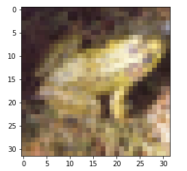
Next, load the tmodel manifest for the model into the driver. The manifest tells the driver where to find the other two binary files (program and weights data).
tcu.load_model('/home/xilinx/resnet20v2_cifar_onnx_ultra96v2.tmodel')
Finally, run the model and print the results! The call to tcu.run(inputs) is where the magic happens. We’ll convert the ResNet classification result vector into CIFAR labels. Note that if you are using the ONNX model, the input and output are named x:0 and Identity:0 respectively. For the TensorFlow model they are named x and Identity.
inputs = {'x:0': img}

start = time.time()
outputs = tcu.run(inputs)
end = time.time()
print("Ran inference in {:.4}s".format(end - start))
print()

classes = outputs['Identity:0'][:10]
result_idx = np.argmax(classes)
result = label_names[result_idx]
print("Output activations:")
print(classes)
print()
print("Result: {} (idx = {})".format(result, result_idx))
print("Actual: {} (idx = {})".format(label, label_idx))
Here is the expected result:
Ran inference in 0.03043s

Output activations:
[-13.59375    -12.25        -7.90625     -6.21484375  -8.25
 -12.24609375  15.0390625  -15.10546875 -10.71875     -9.1796875 ]

Result: frog (idx = 6)
Actual: frog (idx = 6)
Congratulations! You ran a machine learning model a custom ML accelerator that you built on your own work station! Just imagine the things you could do with it…
Wrap-up
In this tutorial we used Tensil to show how to run machine learning (ML) models on FPGA. We went through a number of steps to get here, including installing Tensil, choosing an architecture, generating an RTL design, synthesizing the desing, compiling the ML model and finally executing the model using PYNQ.
If you made it all the way through, big congrats! You’re ready to take things to the next level by trying out your own model and architecture. Join us on Discord to say hello and ask questions, or send an email to [email protected].