Building speech controlled robot with Tensil and Arty A7 - Part I

Originally posted here.

Introduction

In this two-part tutorial we will learn how to build a speech controlled robot using Tensil open source machine learning (ML) acceleration framework and Digilent Arty A7-100T FPGA board. At the heart of this robot we will use the ML model for speech recognition. We will learn how Tensil framework enables ML inference to be tightly integrated with digital signal processing in a resource constrained environment of a mid-range Xilinx Artix-7 FPGA.

Part I will focus on recognizing speech commands through a microphone. Part II will focus on translating commands into robot behavior and integrating with the mechanical platform.

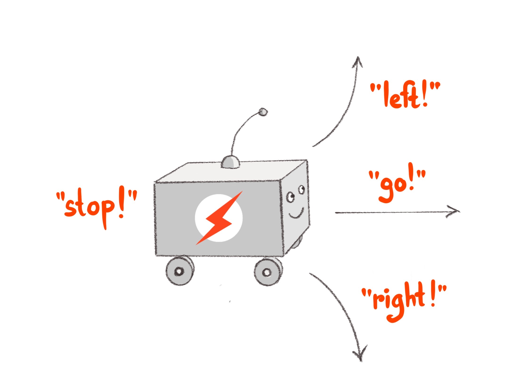
Let’s start by specifying what commands we want the robot to understand. To keep the mechanical platform simple (and inexpensive) we will build on a wheeled chassis with two engines. The robot will recognize directives to move forward in a straight line (go!), turn in-place clockwise (right!) and counterclockwise (left!), and turn the engines off (stop!).

System architecture

Now that we know what robot we want to build, let’s define its high-level system architecture. This architecture will revolve around the Arty board that will provide the “brains” for our robot. In order for the robot to “hear” we need a microphone. The Arty board provides native connectivity with the PMOD ecosystem and there is MIC3 PMOD from Digilent that combines a microphone with ADCS7476 analog-to-digital converter. And in order to control motors we need two HB3 PMOD drivers, also from Digilent, that will convert digital signals to voltage level and polarity to drive the motors. (We also suggest purchasing a 12” or 18” PMOD extender cable for MIC3 for best sound reception.)

Next let’s think about how to structure our system starting with the microphone turning the sound waveform into electrical signals down to controlling the engines speed and direction. There are two independent components emerging.

The first component continuously receives the microphone signal as an input and turns it into events, each representing one of the four commands. Lets call it a Sensor Pipeline. The second component receives a command event and, based on it, changes its state accordingly. This state represents what the robot is currently doing and therefore translates directly into engine control signals. Let’s call this component a State Machine.

In this part of the tutorial we will focus on building the sensor pipeline. In part II we will take on building the state machine plus assembling and wiring it all together.

Another important point of view for system architecture is separation between software and hardware. In the case of the Arty board the software will run on a Xilinx Microblaze processor–which is itself implemented on top of FPGA fabric–a soft CPU. This means that we won’t have the computation power typically available in the hard CPU–the CPU implemented in silicon–and instead should rely on hardware acceleration whenever possible. This means that the CPU should only be responsible for orchestrating various hardware components to do the actual computation. The approach we will be taking is to keep software overhead to an absolute minimum by running a tiny embedded C program that will fit completely into 64K of static memory embedded into an FPGA (BRAM). This program will then use external DDR memory to organize communication between hardware accelerators using Direct Memory Access (DMA).

Sensor pipeline

This chapter will provide a detailed overview of the principles of operation for the sensor pipeline. Don’t worry about the content being on the theoretical side–the next chapter will be step-by-step instructions on how to build it.

Microphone acquisition

The first stage of the sensor pipeline is acquisition of the numeric representation of the sound waveform. Such representation is characterized by the sampling rate. For a sampling rate of 16 KHz the acquisition will produce a number 16,000 times per second. The ADCS7476 analog-to-digital converter is performing this sampling by turning the analog signal from the microphone to a 16-bit digital number. (It is really a 12-bit number with zero padding in most significant bits.) Since we are using the Arty board with Xilinx FPGA, the way to integrate various components in the Xilinx ecosystem is through the AXI4 interface. ADCS7476 converter supports a simple SPI interface, which we adapt to AXI4-Stream with a little bit of Verilog. Once converted to AXI4-Stream we can use standard Xilinx components to convert from 16-bit integer to single precision (32-bit) floating point and then apply fused multiply-add operation in order to scale and offset the sample to be between -1 and 1. One additional function of the acquisition pipeline is to put samples together to form packets of a certain length. This length is 128 samples. Both normalization and the packet length are required by the next stage in the sensor pipeline described below.

Speech commands ML model

At the heart of our sensor pipeline is the machine learning model that given 1 second of sound data predicts if it contains a spoken command word. We based it loosely on TensorFlow simple audio recognition tutorial. If you would like to understand how the model works we recommend reading through it. The biggest change from the original TensorFlow tutorial is using a much larger speech commands dataset. This dataset extends the command classes to contain an unknown command and a silence. Both are important for distinguishing commands we are interested in from other sounds such as background noise. Another change is in the model structure. We added a down-convolution layer that effectively reduces the number of model parameters to make sure it fits the tight resources of Artix-7 FPGA. Lastly, once trained and saved, we convert the model to ONNX format. You can look at the process of training the model in the Jupyter notebook. One more thing to note is that the model supports more commands that we will be using. To work around that the actual state machine component may ignore events for unsupported commands. (And we invite you to extend the robot to take advantage of all of the commands!)

To run this model on an FPGA we will use Tensil. Tensil is an open source ML acceleration framework that will generate a hardware accelerator with a given set of parameters specifying the Tensil architecture. Tensil makes it very easy to compile ML models created with popular ML frameworks for running on this accelerator. There is a good introductory tutorial that explains how to run a ResNet ML model on an FPGA with Tensil. It contains a detailed step-by-step description of building FPGA design for Tensil in Xilinx Vivado and later using it with the PYNQ framework. In this tutorial we will instead focus on system integration as well as aspects of running Tensil in a constrained embedded environment.

For our purpose it is important to note that Tensil is a specialized processor–Tensil Compute Unit (TCU)–with its own instruction set. Therefore we need to initialize it with the program binary (.tprog file). With the Tensil compiler we will compile the commands ONNX model, parametrized by the Tensil architecture, into a number of artifacts. The program binary is one of them.

Another artifact produced by the compiler is the data binary (.tdata file) containing weights from the ML model adapted for running with Tensil. These two artifacts need to be placed in system DDR memory for TCU to be able to read them. One more artifact produced by the Tensil compiler is model description (.tmodel file). This file is usually consumed by the Tensil driver when there is a filesystem available (such as one on a SD card) in order to run the inference with a fewest lines of code.

The Arty board does not have an SD card and therefore we don’t use this approach. Instead we place the program and data binaries into Quad-SPI flash memory along with the FPGA bitstream. At initialization and inference we use values from the model description to work directly with lower level abstractions of the Tensil embedded driver.

The TCU dedicates two distinct memory areas in the DDR to data. One for variables or activations in ML speak–designated DRAM0 for Tensil. Another is for constants or weights–designated DRAM1. Data binary needs to be copied from flash memory to DRAM1 with base and size coming from the model description. Model inputs and outputs are also found in the model description as base and size within DRAM0. Our program will be responsible for writing and reading DRAM0 for every inference. Finally, the program binary is copied into a DDR area called the instruction buffer.

You can take a look at the model description produced by the Tensil compiler and at the corresponding TCU initialization steps in the speech robot source code.

Fourier transform

The TensorFlow simple audio recognition tutorial explains that the ML model does not work directly on the waveform data from the acquisition pipeline. Instead, it requires a sophisticated preprocessing step that runs Short-time Fourier transform (STFT) to get a spectrogram. Good news is that Xilinx has a standard component for Fast Fourier transform (FFT). The FFT component supports full-fledged Fourier transforms with complex numbers as input and output.

The STFT uses what is called Real FFT (RFFT). RFFT augments the FFT by consuming only real numbers and setting the imaginary parts to zero. RFFT produces FFT complex numbers unchanged, which SFTF subsequently turns into magnitudes. The magnitude of a complex number is simply a square root of the sum of the real and imaginary parts both squared. This way, input and output STFT packets have the same number of values.

The STFT requires that the input to RFFT be a series of overlapping windows into the waveform from the acquisition pipeline. Each such window is further augmented by applying a special window function. Our speech commands model uses the Hann window function. Each waveform sample needs to be in the range of -1 and 1 and then multiplied by the corresponding value from the Hann window. Application of the Hann window has an effect of “sharpening” the spectrogram image.

The speech commands model sets the STFT window length to 256 with a step of 128. This is why the acquisition pipeline produces packets of length 128. Each acquisition packet is paired with the previous packet to form one STFT input packet of length 256.

We introduce another bit of Verilog to provide a constant flow of Hann window packets to multiply with waveform packets from the acquisition pipeline.

Finally, the STFT assembles together a number of packets into a frame. The height of this frame is the number of packets that were processed for a given spectrogram, which represents the time domain. Our speech commands model works on a 1 second long spectrogram, which allows for all supported one-word commands to fit. Given a 16 KHz sampling rate, an STFT window length of 256 samples, and a step of 128 samples we get 124 STFT packets that fit into 1 second.

The width of the STFT frame represents the frequency domain in terms of Fourier transform. Furthermore, the 256 magnitudes in the output STFT packets have symmetry intrinsic to RFFT that allows us to take the first 129 values and ignore the rest. Therefore the input frame used for the inference is 129 wide and 124 high.

Since STFT frame magnitudes are used as an input to the inference we need to convert them from single precision (32-bit) floating point to 16-bit fixed point with 8-bit base point (FP16BP8). FP16BP8 is one of the data types supported by Tensil that balances sufficient precision with good memory efficiency and enables us to avoid quantizing the ML model in most cases. Once again, we reach for various Xilinx components to perform AXI4-Stream manipulation and mathematical operations on a continuous flow of packets through STFT pipeline.

Softmax

The speech commands model outputs its prediction as a vector with a value for each command. It is generally possible to find the greatest value and therefore tell from its position which command was inferred. This is the argmax function. But in our case we also need to know the “level of confidence” in this result. One way of doing this is using the softmax function on the prediction vector to produce 0 to 1 probability for each command, which will sum up to 1 for all commands. With this number we can more easily come up with a threshold on which the sensor pipeline will issue the command event.

In order to compute the softmax function we need to calculate the exponent for each value in the prediction vector. This operation can be slow if implemented in software and following our approach we devise yet another acceleration pipeline. This pipeline will convert FP16BP8 fixed-point format into double precision (64-bit) floating point and perform exponent function on it. The pipeline’s input and output packet lengths are equal to the length of the prediction vector (12). The output is written as double precision floating point for the software to perform final summation and division.

The main loop

As you can see the sensor pipeline consists of a number of distinct hardware components. Namely we have acquisition followed by STFT pipeline, followed by Tensil ML inference, followed by softmax exponent pipeline. The Microblaze CPU needs to orchestrate their interaction by ensuring that they read and write data in the DDR memory without data races and ideally without the need for extra copying.

This pipeline also defines what is called a main loop in the embedded system. Unlike conventional software programs, embedded programs, once initialized, enter an infinite loop through which they continue to operate indefinitely. In our system this loop has a hard deadline. Once we receive a packet of samples from the acquisition pipeline we need to immediately request the next one. If not done quickly enough the acquisition hardware will drop samples and we will be getting a distorted waveform. In other words as we loop through acquisition of packets each iteration can only run for the time it takes to acquire the current packet. At 16 KHz and 128 samples per packet this is 8 ms.

The STFT spectrogram and softmax exponent components are fast enough to take only a small fraction of 8ms iteration. Tensil inference is much more expensive and for the speech model it takes about 90ms (the TCU clocked at 25 MHz.) But the inference does not have to happen for every acquisition packet. It needs to have the entire spectrogram frame that is computed from 124 packets, which add up to 1 second! So, can the inference happen every second with plenty of time to spare? It turns out that if the model “looks” at consecutive spectrograms the interesting pattern can be right on the edge where both inferences will not recognize it. The solution is to run the inference on the sliding window over the spectrogram. This way if we track 4 overlapping windows over the spectrogram we can run inference every 250 ms and have plenty of opportunity to recognize interesting patterns!

Let’s summarize the main loop in the diagram below. The diagram also includes the 99% percentile (worst case) time it takes for each block to complete so we keep track of the deadline.

You can look at the main loop in the speech robot source code.

Assembling the bits

Now let’s follow the steps to actually create all the bits necessary for running the sensor pipeline. Each section in this chapter describes necessary tools and source code to produce certain artifacts. At the end of each section there is a download link to the corresponding ready-made artifacts. It’s up to you to follow the steps to recreate it yourself or skip and jump directly to your favorite part!

Speech commands model

We’ve already mentioned the Jupyter notebook with all necessary steps to download the speech commands dataset, train and test the model, and convert it to ONNX format. For dataset preprocessing you will need the ffprobe tool from the ffmpeg package on Debian/Ubuntu. Even though the model is not very large we suggest using GPU for training. We also put the resulting speech commands model ONNX file in the GitHub at the location where the Tensil compiler from the next section expects to find it.

Tensil RTL and model

Next step is to produce the Register Transfer Level (RTL) representation of Tensil processor–the TCU. Tensil tools are packaged in the form of Docker container, so you’ll need to have Docker installed and then pull Tensil Docker image by running the following command.

docker pull tensilai/tensil

Launch Tensil container in the directory containing our speech robot GitHub repository by running.

docker run -u $(id -u ${USER}):$(id -g ${USER}) -v $(pwd):/work -w /work -it tensilai/tensil bash

Now we can generate RTL Verilog files by running the following command. Note that we use -a argument to point to Tensil architecture definition, -d argument to request TCU to have 128-bit AXI4 interfaces, and -t to specify the target directory.

tensil rtl -a ./arch/speech_robot.tarch -d 128 -t vivado

The RTL tool will produce 3 new Verilog (.v) files in the vivado directory: top_speech_robot.v contains the bulk of generated RTL for the TCU. bram_dp_128x2048.v and bram_dp_128x8192.v encapsulate RAM definitions to help Vivado to infer the BRAM. It will also produce architecture_params.h containing Tensil architecture definition in the form of a C header file. We will use it to initialize the TCU in the embedded application.

All 4 files are already included in the GitHub repository.

The final step in this section is to compile the ML model to produce the artifacts that TCU will use to run it. This is accomplished by running the following command. Again we use -a argument to point to Tensil architecture definition. We then use -m argument to point to speech commands model ONNX file, -o to specify the name of the output node in the ONNX graph (you can inspect this graph by opening the ONNX file in the Netron), and -t to specify the target directory.

tensil compile -a ./arch/speech_robot.tarch -m ./model/speech_commands.onnx -o "dense_1" -t model

The compiler will produce program and data binaries (.tprog and .tdata files) along with the model description (.tmodel file). First two will be used in the step where we build a flash image file. Model description will provide us with important values to initialize the TCU in the embedded application.

All 3 files are also included in the GitHub repository.

Vivado bitstream

Now that we have prepared the RTL sources it is time to synthesize the hardware! In the FPGA world this means creating a bitstream to initialize the FPGA fabric so that it turns into our hardware. For Xilinx specifically, this also means bundling the bitstream with all of the configuration necessary to initialize software drivers into a single Xilinx Shell Archive (XSA) file.

We will be using Vivado 2021.1, which you can download and use for free for educational projects. Make sure to install Vitis, which will include Vivado and Vitis. We will use Vitis in the next section when building the embedded application for the speech robot.

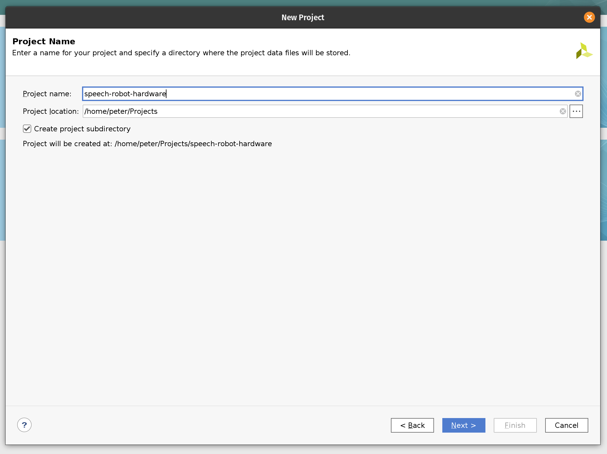
We start by creating a new Vivado project. Let’s name it speech-robot-hardware.

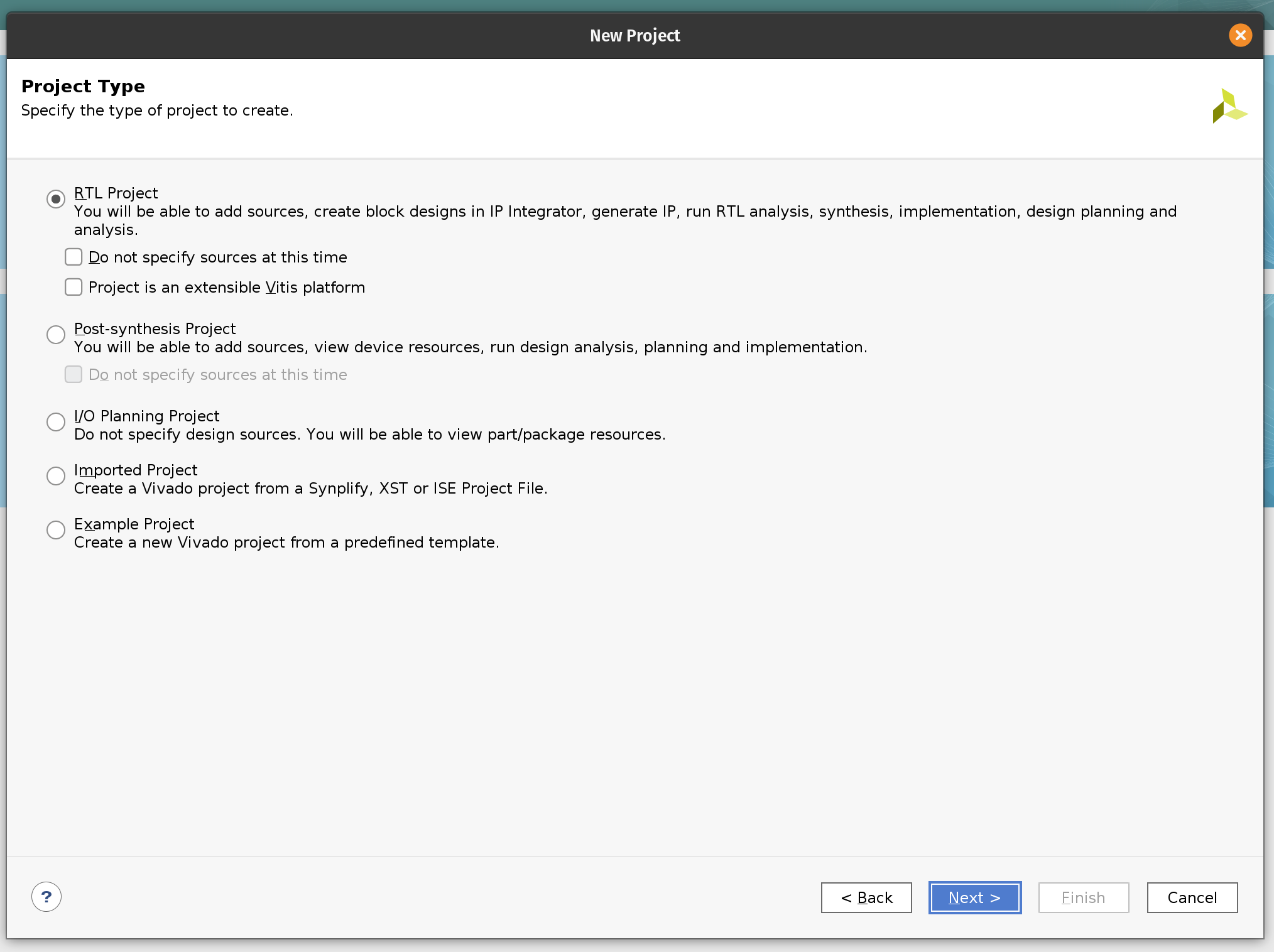
Next, we select the project type to be an RTL project.

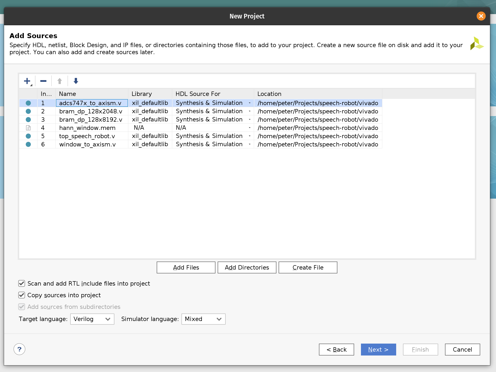
On the next page, add Verilog files and the hann_window.mem file with ROM content for the Hann window function.

Next, add the Arty-A7-100-Master.xdc constraint file. We use this constraint file to assign the pins of the FPGA chip. The upper part of the JB PMOD interface is connected to the MIC3 module. The upper parts of the JA and JD PMOD interfaces are connected the left and right motor’s HB3 modules correspondingly.

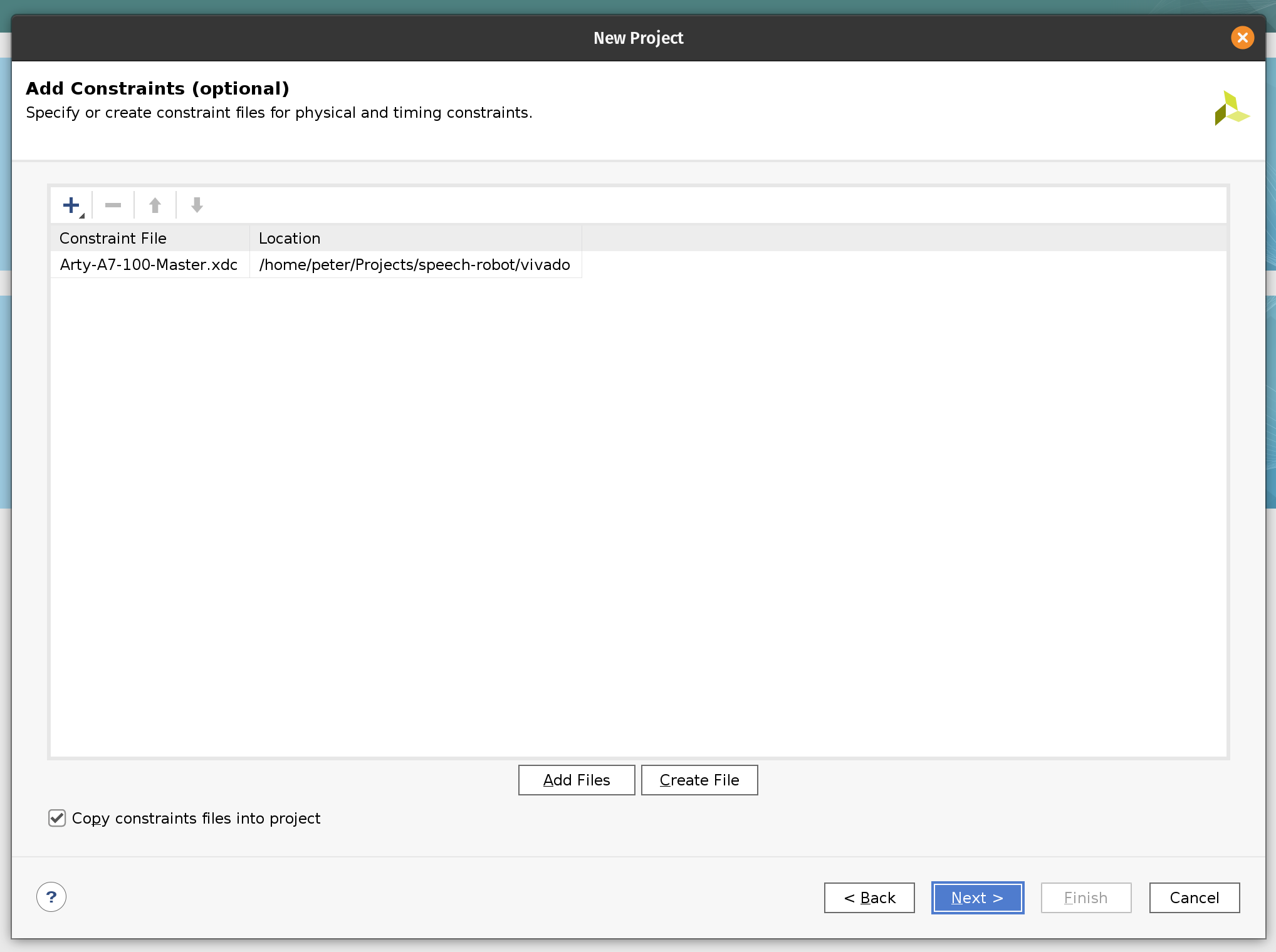
The next page will allow us to select the target FPGA board. Search for “Arty” and select Arty A7-100. You may need to install the board definition by clicking on the icon in the Status column.

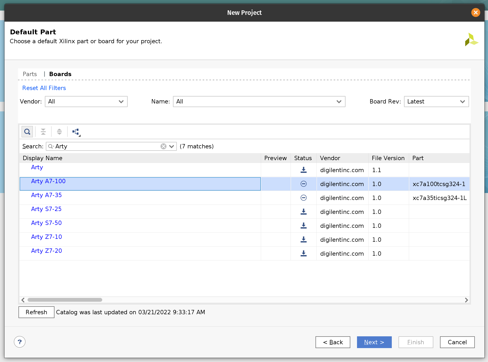
Click Next and Finish.

Next we need to import the Block Design. This will instantiate and configure the RTL we imported and many standard Xilinx components such as MicroBlaze, FFT and the DDR controller. The script then will wire everything together. In our previous Tensil tutorials we included step-by-step instructions on how to build Block Design from ground up. It was possible because the design was relatively simple. For the speech robot the design is a lot more complex. To save time we exported it from Vivado as a TCL script, which we now need to import.

To do this you will need to open the Vivado TCL console. (It should be one of the tabs at the bottom of the Vivado window.) Once in the console run the following command. Make sure to replace /home/peter/Projects/speech-robot with the path to the cloned GitHub repository.

source /home/peter/Projects/speech-robot/vivado/speech_robot.tcl

Once imported, right click on the speech_robot item in the Sources tab and then click on Create HDL Wrapper. Next choose to let Vivado manage wrapper and auto-update.

Once Vivado created the HDL wrapper the speech_robot item will get replaced with speech_robot_wrapper. Again, right click on it and then click Set as Top.

You should now be able to see the entire Block Design. (Image is clickable.)

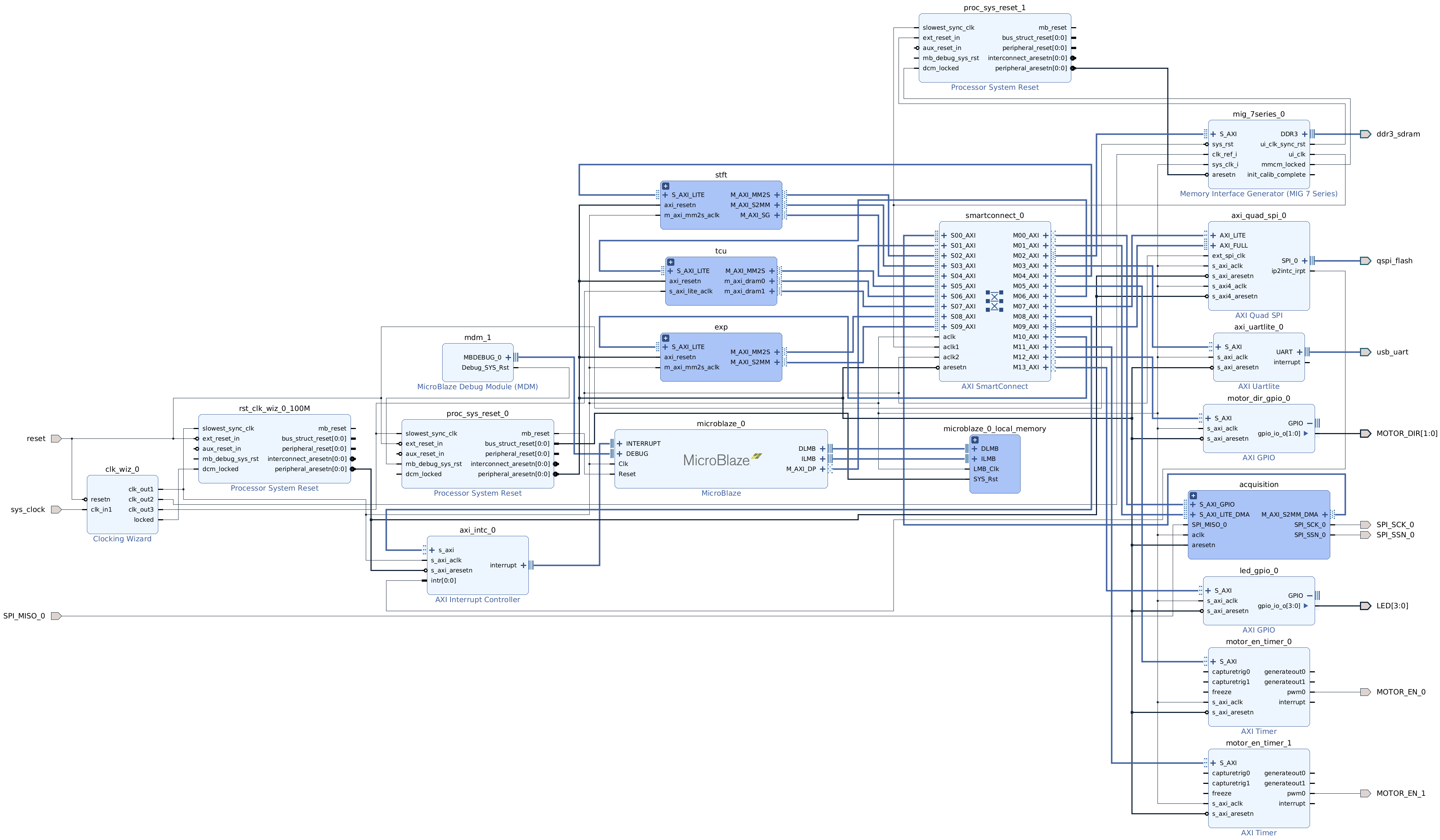
There are hierarchies (darker blue blocks) that correspond to our acceleration pipelines. These hierarchies are there to make the top-level diagram manageable. If you double-click on one of them they will open as a separate diagram. You can see that what is inside closely resembles diagrams from the discussion in the previous chapter.

Let’s peek into the STFT pipeline. You can see Hann window multiplication on the left, followed by the Xilinx FFT component in the middle, followed by the magnitude and fixed point conversion operations on the right.

Similarly for acquisition and exponent pipelines.

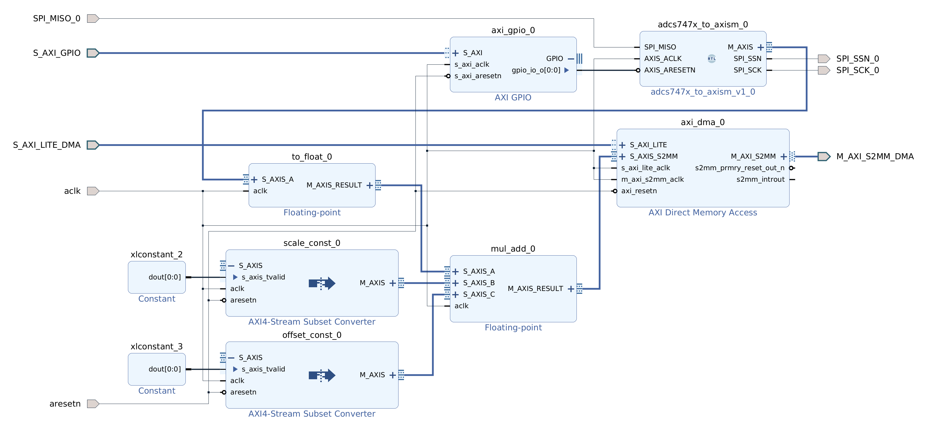
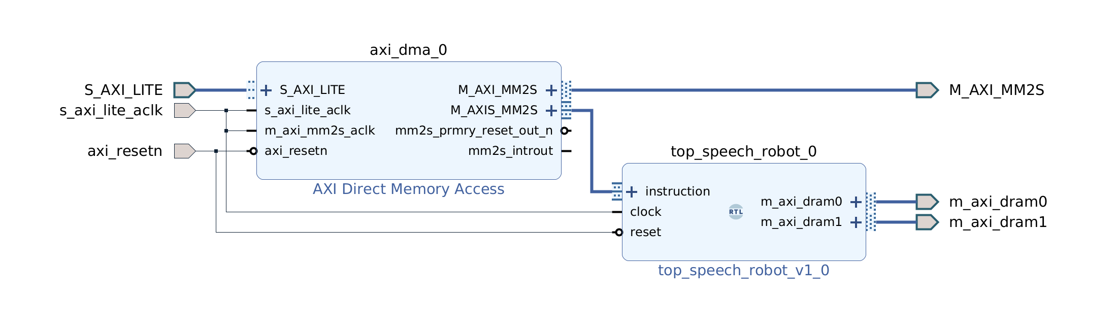
Design for the TCU hierarchy is very simple. We need an AXI DMA component to feed the program to the AXI4-Stream instruction port. DRAM0 and DRAM1 are full AXI ports and therefore go directly to the interconnect.

Now it’s time to synthesize the hardware. In the left-most pane click on Generate Bitstream, then click Yes and OK to launch the run. Now is a good time for a break!

Once Vivado finishes its run, the last step is to create the XSA file. Click on the File menu and then click Export and Export Hardware. Make sure that the XSA file includes the bitstream.

If you would like to skip the Vivado steps we included the XSA file in the GitHub repository.

Vitis embedded application

In this section we will follow the steps to build the software for the speech robot. We will use the Tensil embedded driver to interact with the TCU and the Xilinx AXI DMA driver to interact with other acceleration pipelines.

The entire application is contained in a single source code file. The comments contain further details that are not covered here. We highly recommend browsing through this file so that the rest of the tutorial makes more sense.

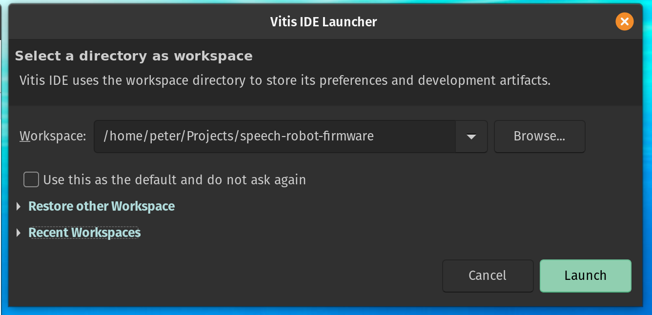
Let’s start by launching the Vitis IDE which prompts us to create a new workspace. Lets call it speech-robot-firmware.

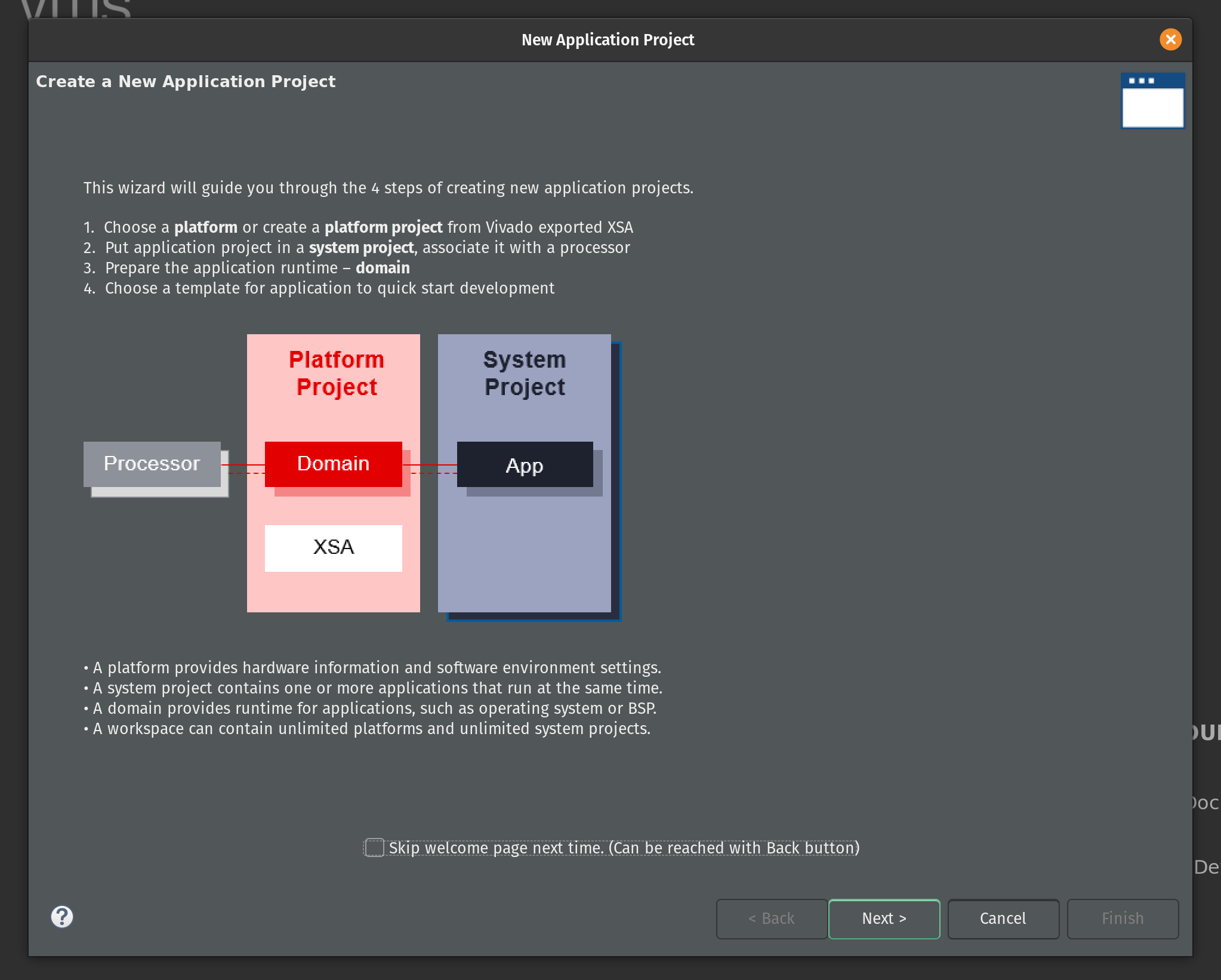
On the Vitis welcome page click Create Application Project. The first page of the New Application Project wizard explains what is going to happen. Click Next.

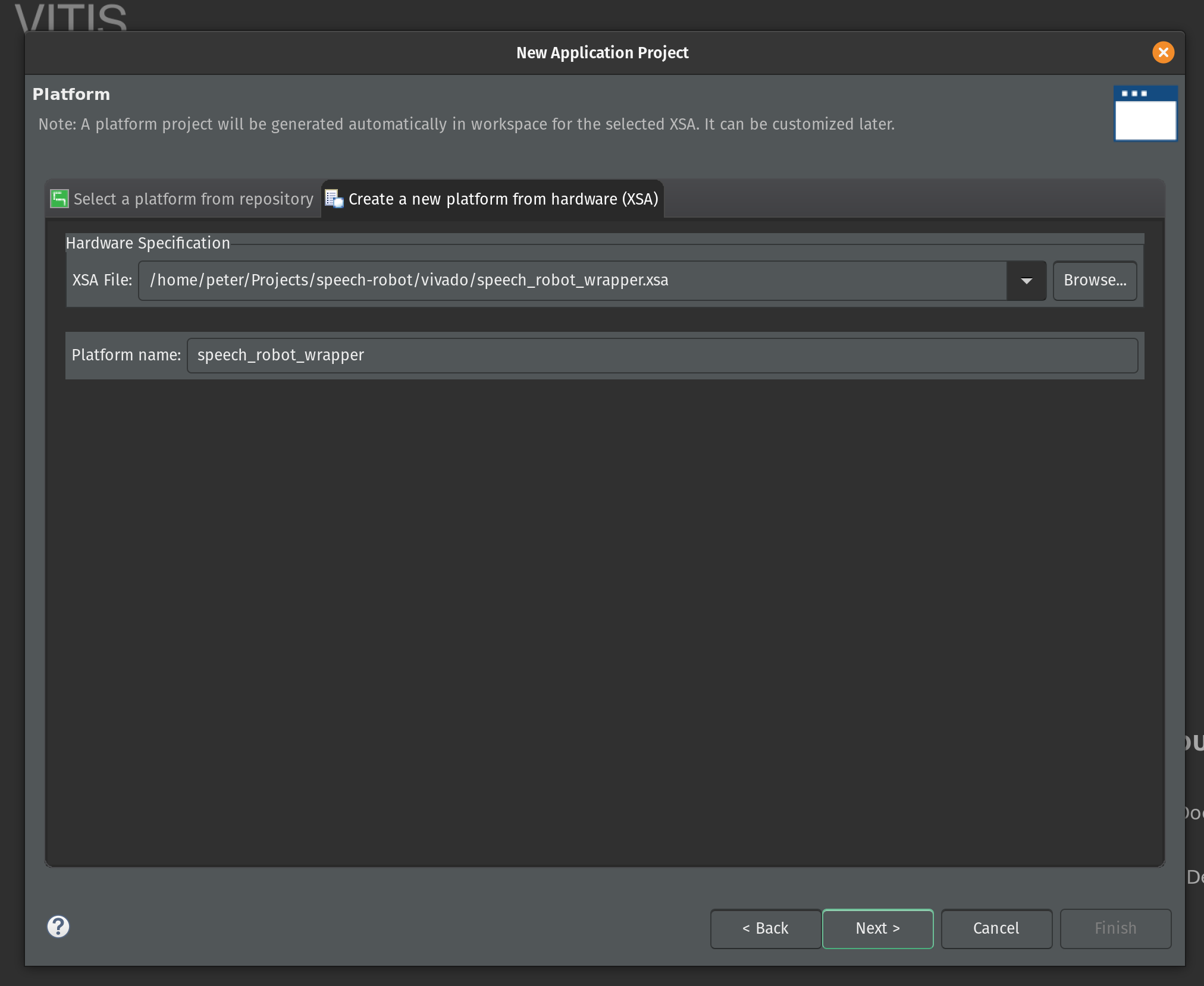
Now select Create a new platform from hardware (XSA) and select the location of the XSA file. Click Next.

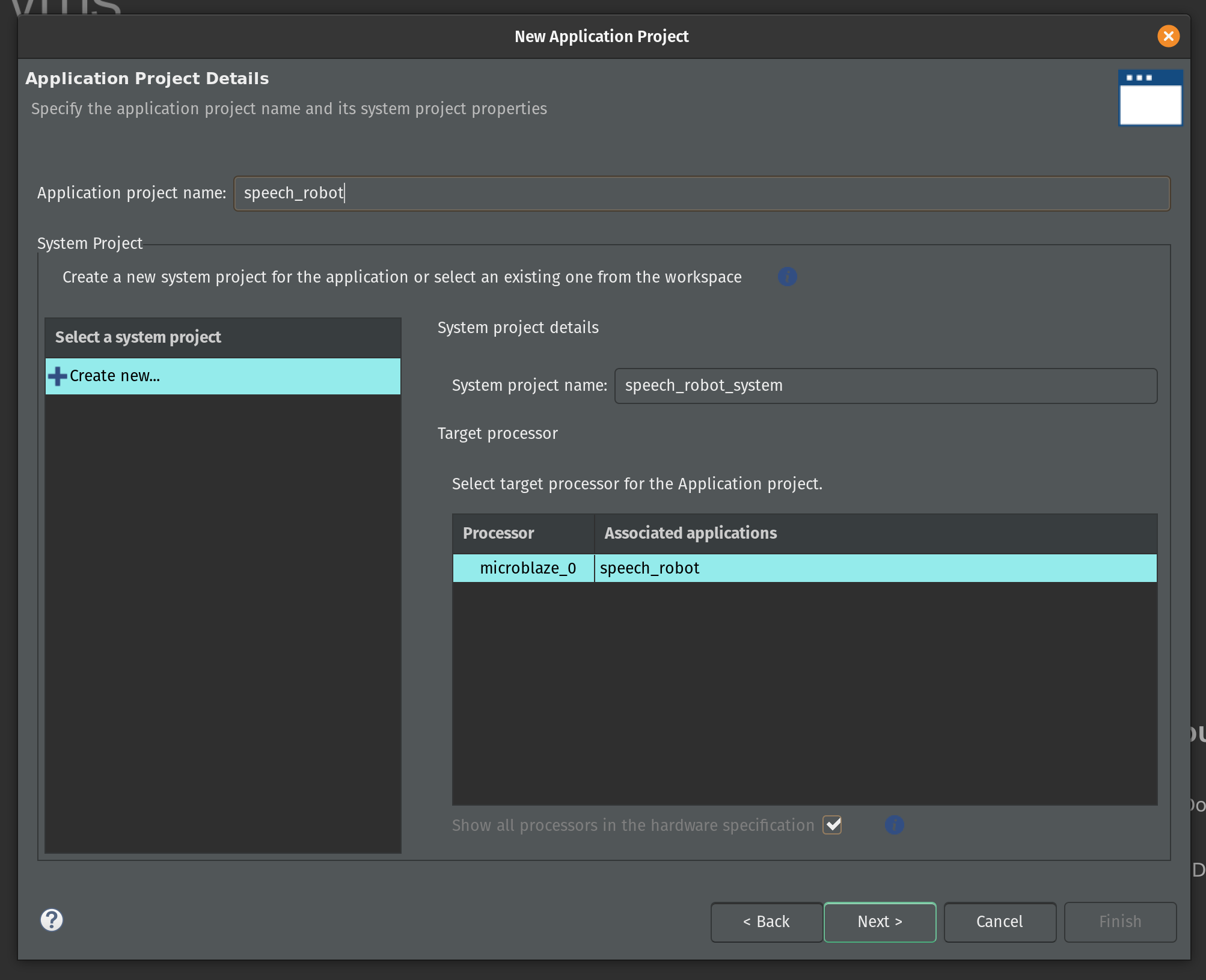
Enter the name for the application project. Type in speech_robot and click Next.

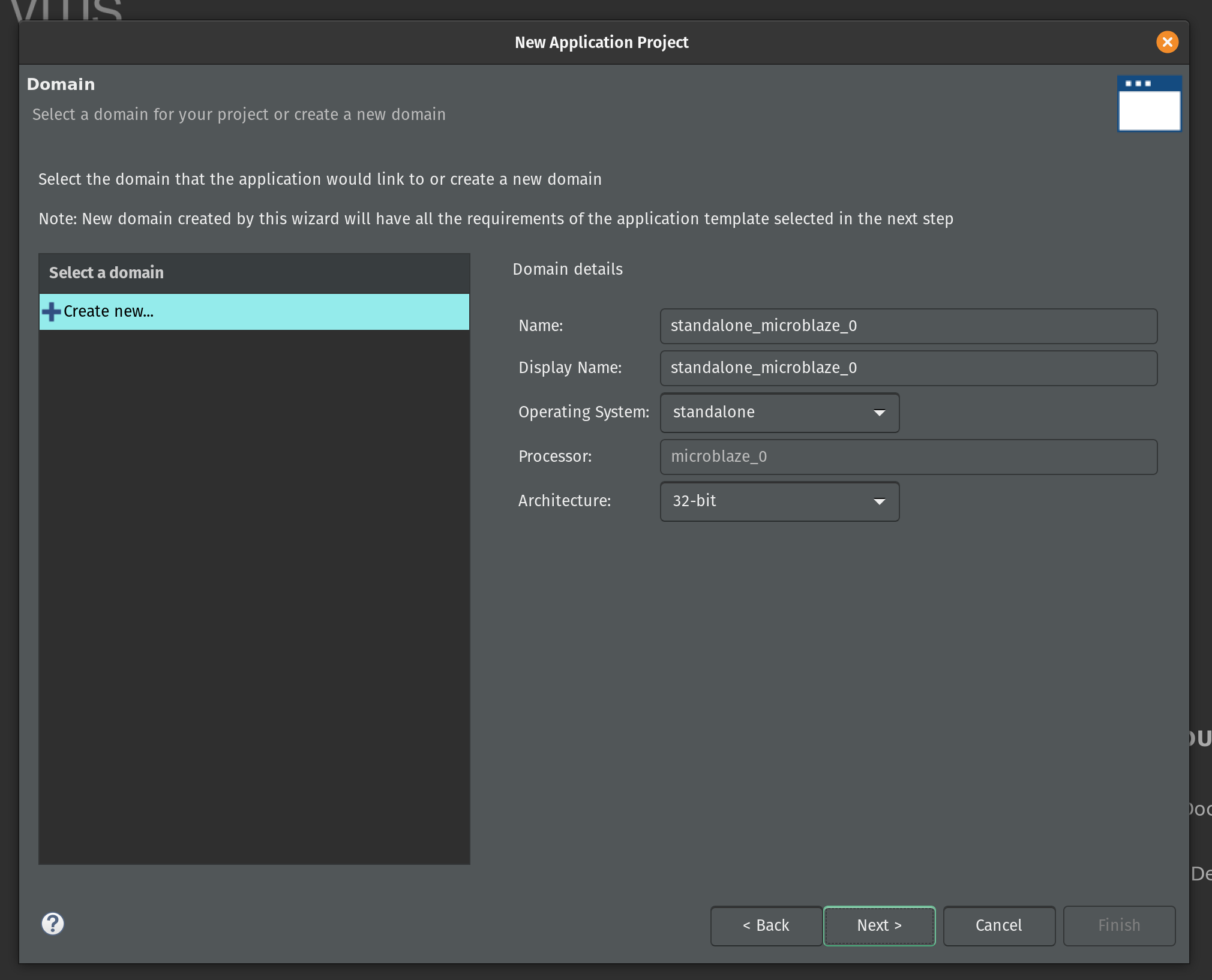
On the next page keep the default domain details unchanged and click Next.

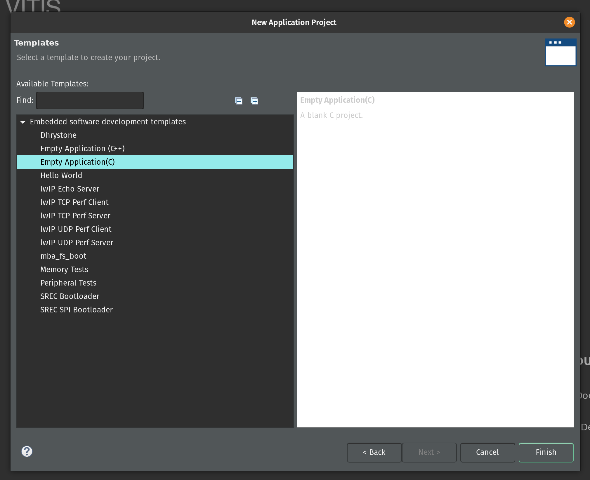
Select the Empty Application (C) as a template and click Finish.

Vitis created two projects in our workspace. The speech_robot_wrapper is a platform project that contains drivers and other base libraries configured for our specific hardware. This project is based on the XSA file and every time we change the XSA in Vivado we will need to update and rebuild the platform project.

The second is the system project speech_robot_system. The system project exposes tools to create boot images and program flash. (We’ll use Vivado for these functions instead.) The system project has an application subproject speech_robot. This project is what we will be populating with source files and building.

Let’s start by copying the source code for speech robot from its GitHub repository. The following commands assume that this repository and the Vitis workspace are on the same level in the file system.

cp speech-robot/vitis/speech_robot.c speech-robot-firmware/speech_robot/src/
cp speech-robot/vitis/lscript.ld speech-robot-firmware/speech_robot/src/
cp speech-robot/vivado/architecture_params.h speech-robot-firmware/speech_robot/src/

Next we need to clone Tensil repository and copy the embedded driver source code.

git clone [https://github.com/tensil-ai/tensil](https://github.com/tensil-ai/tensil)
cp -r tensil/drivers/embedded/tensil/ speech-robot-firmware/speech_robot/src/

Finally we copy one last file from the speech robot GitHub repository that will override the default Tensil platform definition.

cp speech-robot/vitis/tensil/platform.h speech-robot-firmware/speech_robot/src/tensil/

Now that we have all source files in the right places lets compile and link our embedded application. In the Assistant window in the left bottom corner click on Release under speech_robot [Application] project and then click Build.

This will generate an executable ELF file located in speech_robot/Release/speech_robot.elf under the Vitis workspace directory.

If you would like to skip the Vitis steps we included the ELF file in the GitHub repository.

Quad-SPI flash image

We now built both hardware (in the form of Vivado bitstream) and software (in the form of ELF executable file.) In this second to final section we will be combining them together with ML model artifacts to create the binary image for the flash memory.

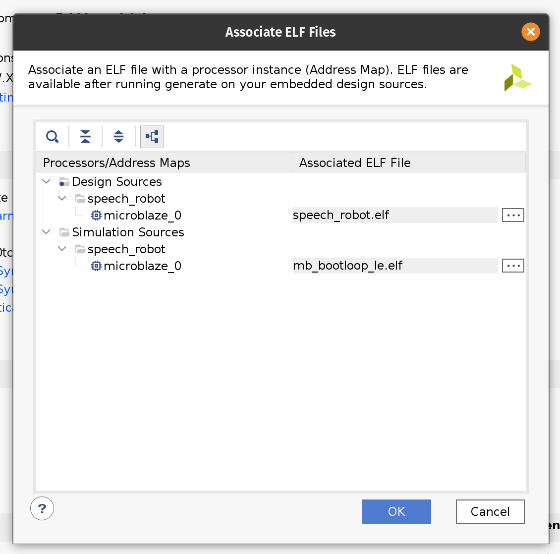
Firstly we need to update the bitstream with an ELF file containing our firmware. By default Vivado fills the Microblaze local memory with the default bootloader. To replace it go to the Tools menu and click Associate ELF files. Then click on the button with three dots and add the ELF file we produced in the previous section. Select it and click OK. Then click OK again.

Now that we changed the ELF file we need to rebuild the bitstream. Click the familiar Generate Bitstream in the left-side pane and wait for the run to complete.

Now we have a new bitstream file that has our firmware baked in!

Plug the Arty board into USB on your computer and then click Open Target under Open Hardware Manager and select Auto Connect.

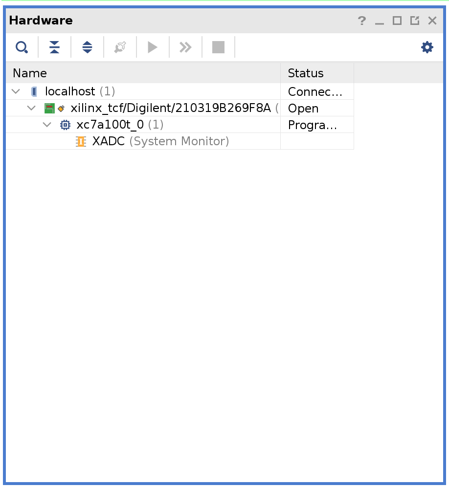
Right-click on xc7a100t_0 and then click Add Configuration Memory Device. Search for s25fl128sxxxxxx0 and select the found part and click OK.

If prompted to program the configuration memory device, click Cancel.

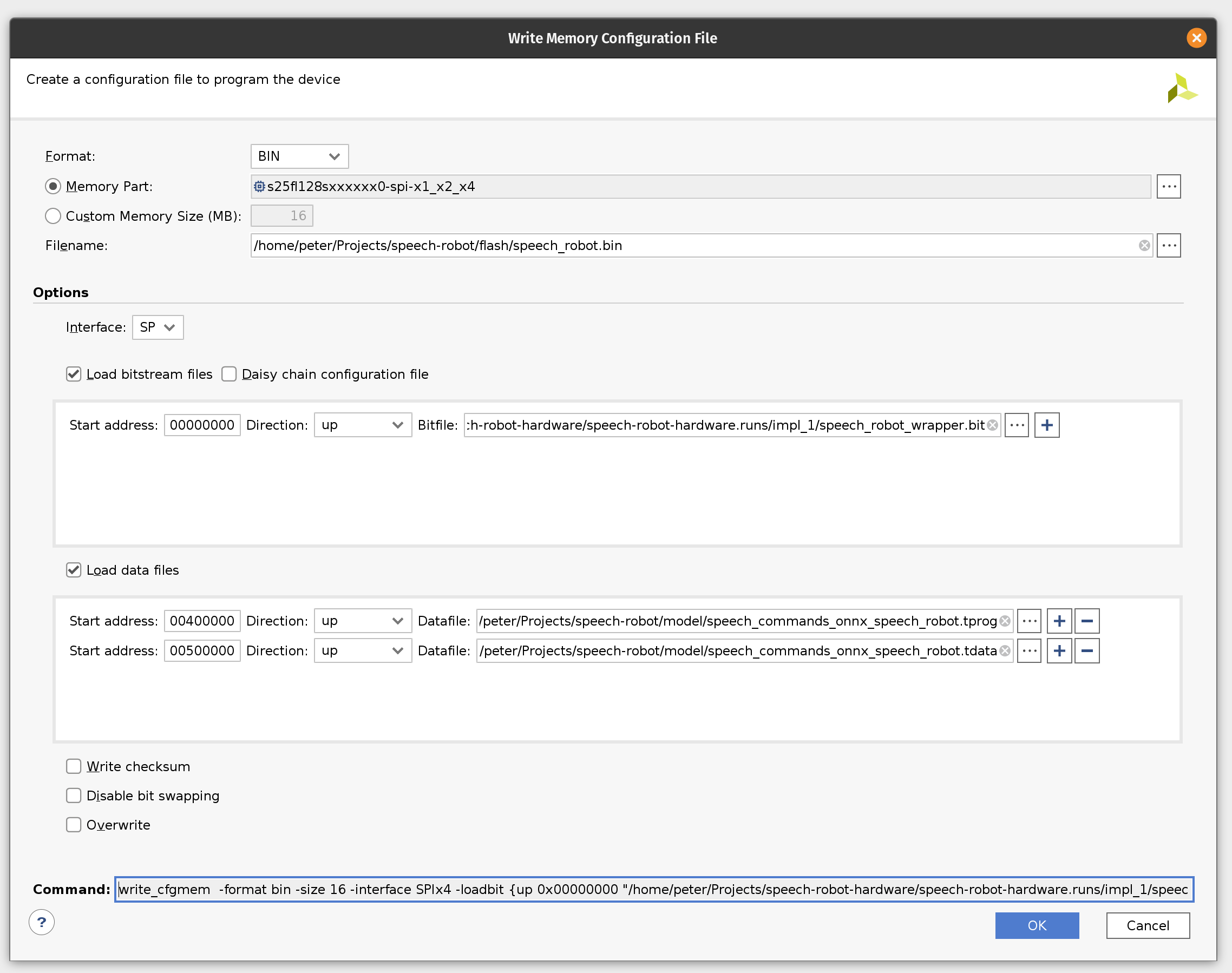
Click on the Tools menu and then click Generate Memory Configuration file. Choose the BIN format and select the available memory part. Enter filename for the flash memory image. (If you are overwriting the existing file, click the Overwrite checkbox at the bottom.)

Next, select the SPIx4 interface. Check the Load bitstream files and enter the location of the bitstream file. (It should be contained in speech-robot-hardware.runs/impl_1/ under the Vivado project directory.

Next, check the Load data files. Set the start address to 00400000 and enter the location of speech_commands_onnx_speech_robot.tprog file. Then click the plus icon. Set the next start address to 00500000 and enter the location of the speech_commands_onnx_speech_robot.tdata file. (Both files should be under the model directory in the GitHub repository.)

Click OK to generate the flash image BIN file.

If you would like to skip all the way to programming we included the BIN file in the GitHub repository.

Programming

In this final (FINAL!!!) section we’ll program the Arty board flash memory and should be able to run the sensor pipeline. The sensor pipeline will print every prediction to the UART device exposed via USB.

Plug the Arty board into USB on your computer and then click Open Target under Open Hardware Manager and select Auto Connect.

If you skipped the previous section where we were creating the flash image BIN file you will need to add the configuration memory device in the Hardware Manager. To do this right-click on xc7a100t_0 and then click Add Configuration Memory Device. Search for s25fl128sxxxxxx0 and select the found part and click OK. If prompted to program the configuration memory device, click OK.

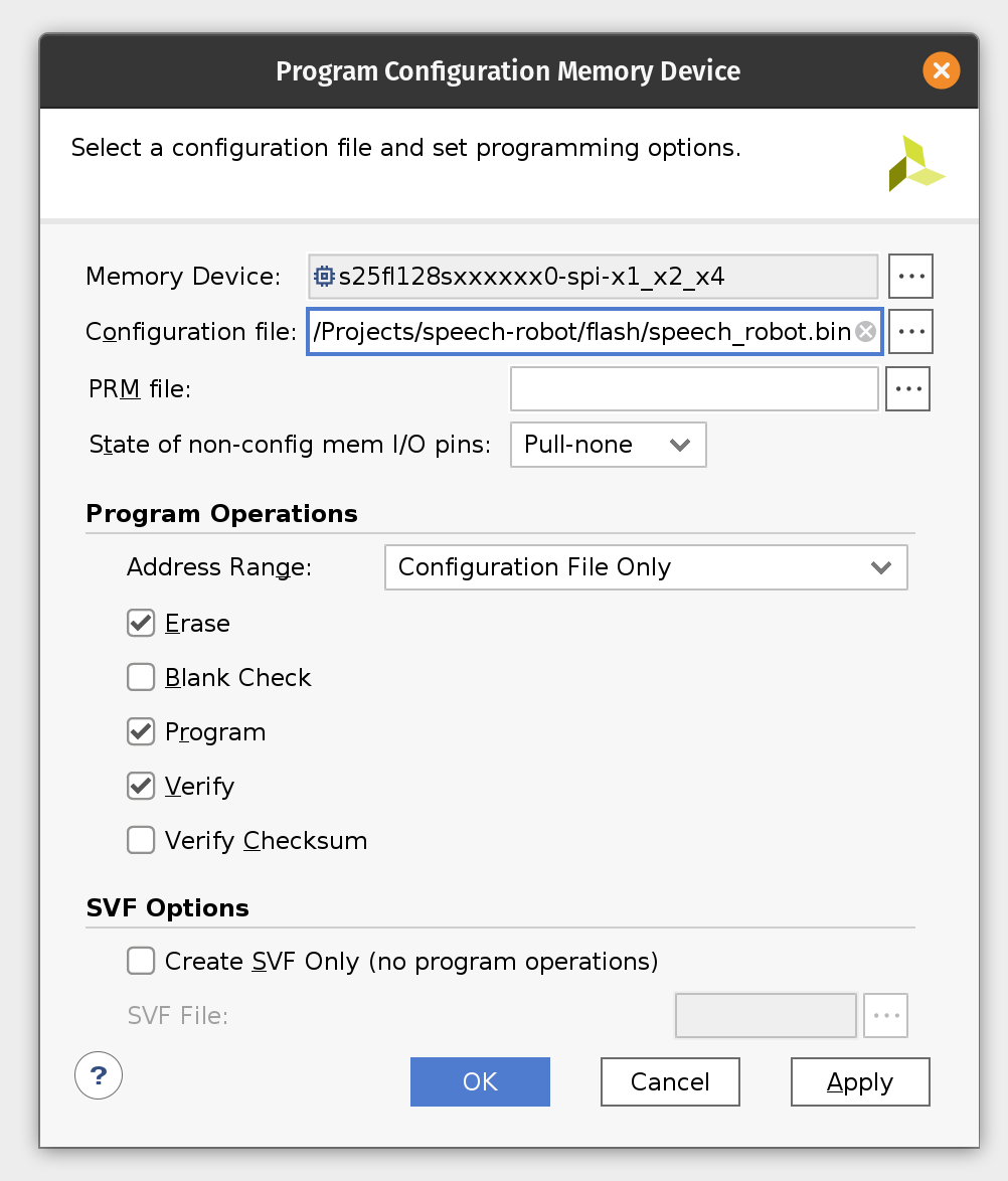
Otherwise right-click on s25fl128sxxxxxx0-spi-x1_x2_x4 and then click Program Configuration Memory Device. Enter the location of the flash image BIN file.

Click OK to program Arty flash.

Now make sure to close Vivado Hardware Manager, otherwise it will interfere with Arty booting from flash and disconnect the board from USB. Connect MIC3 module to the upper part of the JB PMOD interface.

Start the serial IO tool of your choice (like tio) and connect to /dev/ttyUSB1 at 115200 baud. It could be a different device depending on what else is plugged into your computer. Look for a device name starting with Future Technology Devices International.

tio -b 115200 /dev/ttyUSB1

Plug the Arty board back into USB and start shouting commands into your microphone!

The firmware will continuously print the latest prediction starting with its probability. When the event is handled by the State Machine it will add an arrow to highlight this.

0.986799860 _unknown_
0.598671191 _unknown_
0.317275269 up
0.884807667 _unknown_
0.894345367 _unknown_
0.660748154 go <<<
0.924147147 _unknown_
0.865093639 _unknown_
0.725528655 _silence_
0.959776973 _silence_
0.999572298 _silence_
0.993321552 _silence_
0.814953217 _unknown_
0.999999964 left <<<
0.999999981 left
0.999330031 _silence_
0.957002786 _silence_
0.704546136 _unknown_
0.913633790 right <<<
0.974430744 right
0.995242088 right
0.960198592 _silence_
0.870040107 _silence_
0.556416329 stop
0.919281920 _silence_
0.982788728 stop <<<
0.999821720 _silence_
0.913016908 _silence_
0.797638716 _silence_
0.610615039 _unknown_
0.623989887 _unknown_

Conclusion

In the part I of this tutorial we learned how to design an FPGA-based sensor pipeline that combines machine learning and digital signal processing (DSP). We used Tensil open source ML acceleration framework for ML part of the workload and the multitude of standard Xilinx components to implement DSP acceleration. Throughout the tutorial we saw Tensil work well in a very constrained environment of the Microblaze embedded application. Tensil’s entire driver along with the actual application fit in 64 KB of local Microblaze memory. We also saw Tensil integrate seamlessly with the standard Xilinx components, such as FFT, by using shared DDR memory, DMA and fixed point data type.

In part II we will learn how to design the state machine component of the robot and how to interface with motor drivers. Then we will switch from bits to atoms and integrate the Arty board and PMOD modules with the chassis, motors and on-board power distribution.