Learn Tensil with ResNet and PYNQ Z1
Originally posted here.
Introduction
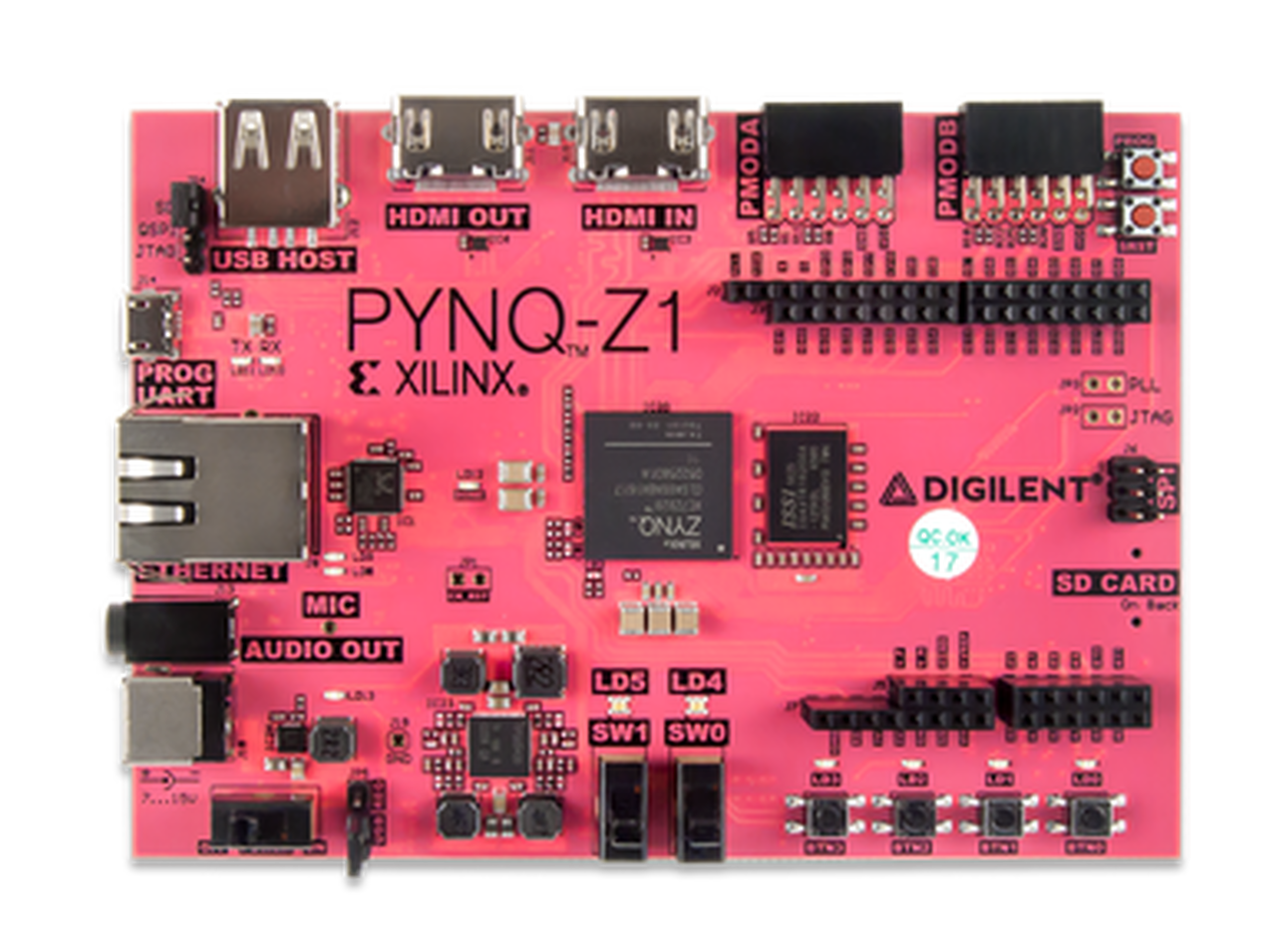
This tutorial will use the PYNQ Z1 development board and Tensil’s open-source inference accelerator to show how to run machine learning (ML) models on FPGA. We will be using ResNet-20 trained on the CIFAR dataset. These steps should work for any supported ML model – currently all the common state-of-the-art convolutional neural networks are supported. Try it with your model!
We’ll give detailed end-to-end coverage that is easy to follow. In addition, we include in-depth explanations to get a good understanding of the technology behind it all, including the Tensil and Xilinx Vivado toolchains and PYNQ framework.
If you get stuck or find an error, you can ask a question on our Discord or send an email to [email protected].
Overview
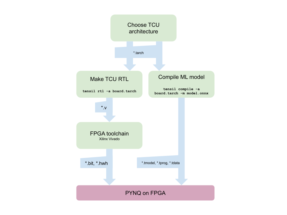
Before we start, let’s look at the Tensil toolchain flow to get a bird’s eye view of what we want to accomplish. We’ll follow these steps:
- Get Tensil
- Choose architecture
- Generate TCU accelerator design (RTL code)
- Synthesize for PYNQ Z1
- Compile ML model for TCU
- Execute using PYNQ
1. Get Tensil
First, we need to get the Tensil toolchain. The easiest way is to pull the Tensil docker container from Docker Hub. The following command will pull the image and then run the container.
docker pull tensilai/tensil
docker run -v $(pwd):/work -w /work -it tensilai/tensil bash
2. Choose architecture
Tensil’s strength is customizability, making it suitable for a very wide range of applications. The Tensil architecture definition file (.tarch) specifies the parameters of the architecture to be implemented. These parameters are what make Tensil flexible enough to work for small embedded FPGAs as well as large data-center FPGAs. Our example will select parameters that provide the highest utilization of resources on the XC7Z020 FPGA part at the core of the PYNQ Z1 board. The container image conveniently includes the architecture file for the PYNQ Z1 development board at /demo/arch/pynqz1.tarch. Let’s take a look at what’s inside.
{
    "data_type": "FP16BP8",
    "array_size": 8,
    "dram0_depth": 1048576,
    "dram1_depth": 1048576,
    "local_depth": 8192,
    "accumulator_depth": 2048,
    "simd_registers_depth": 1,
    "stride0_depth": 8,
    "stride1_depth": 8
}
The file contains a JSON object with several parameters. The first, data_type, defines the data type used throughout the Tensor Compute Unit (TCU), including in the systolic array, SIMD ALUs, accumulators, and local memory. We will use 16-bit fixed-point with an 8-bit base point (FP16BP8), which in most cases allows simple rounding of 32-bit floating-point models without the need for quantization. Next, array_size defines a systolic array size of 8x8, which results in 64 parallel multiply-accumulate (MAC) units. This number was chosen to balance the utilization of DSP units available on XC7Z020 in case you needed to use some DSPs for another application in parallel, but you could increase it for higher performance of the TCU.
With dram0_depth and dram1_depth, we define the size of DRAM0 and DRAM1 memory buffers on the host side. These buffers feed the TCU with the model’s weights and inputs, and also store intermediate results and outputs. Note that these memory sizes are in number of vectors, which means array size (8) multiplied by data type size (16-bits) for a total of 128 bits per vector.
Next, we define the size of the local and accumulator memories which will be implemented on the FPGA fabric itself. The difference between the accumulators and the local memory is that accumulators can perform a write-accumulate operation in which the input is added to the data already stored, as opposed to simply overwriting it. The total size of accumulators plus local memory is again selected to balance the utilization of BRAM resources on XC7Z020 in case resources are needed elsewhere.
With simd_registers_depth, we specify the number of registers included in each SIMD ALU, which can perform SIMD operations on stored vectors used for ML operations like ReLU activation. Increasing this number is only needed rarely, to help compute special activation functions. Finally, stride0_depth and stride1_depth specify the number of bits to use for enabling “strided” memory reads and writes. It’s unlikely you’ll ever need to change this parameter.
3. Generate TCU accelerator design (RTL code)
Now that we’ve selected our architecture, it’s time to run the Tensil RTL generator. RTL stands for “Register Transfer Level” – it’s a type of code that specifies digital logic stuff like wires, registers and low-level logic. Special tools like Xilinx Vivado or yosys can synthesize RTL for FPGAs and even ASICs.
To generate a design using our chosen architecture, run the following command inside the Tensil toolchain docker container:
tensil rtl -a /demo/arch/pynqz1.tarch -s true
This command will produce several Verilog files listed in the ARTIFACTS table printed out at the end. It also prints the RTL SUMMARY table with some of the essential parameters of the resulting RTL.
----------------------------------------------------------------------
RTL SUMMARY
----------------------------------------------------------------------
Data type:                                      FP16BP8
Array size:                                     8
Consts memory size (vectors/scalars/bits):      1,048,576 8,388,608 20
Vars memory size (vectors/scalars/bits):        1,048,576 8,388,608 20
Local memory size (vectors/scalars/bits):       8,192     65,536    13
Accumulator memory size (vectors/scalars/bits): 2,048     16,384    11
Stride #0 size (bits):                          3
Stride #1 size (bits):                          3
Operand #0 size (bits):                         16
Operand #1 size (bits):                         24
Operand #2 size (bits):                         16
Instruction size (bytes):                       8
----------------------------------------------------------------------
4. Synthesize for PYNQ Z1
It is now time to start Xilinx Vivado. I will be using version 2021.2, which you can download free of charge (for prototyping) at the Xilinx website.
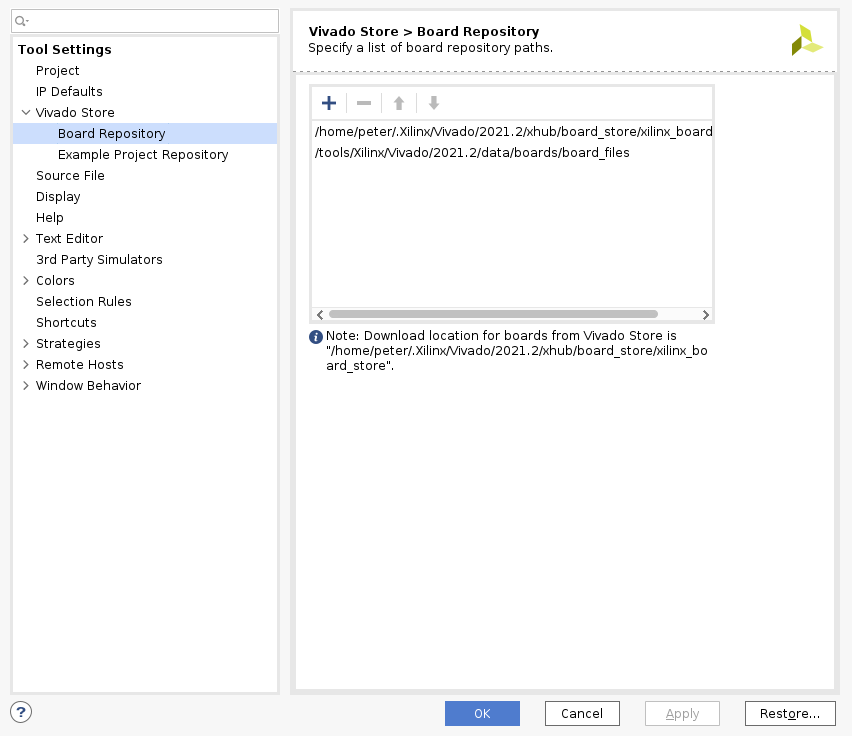
Before you create new Vivado project you will need to download PYNQ Z1 board definition files from here. Unpack and place them in /tools/Xilinx/Vivado/2021.2/data/boards/board_files/. (Note that this path includes Vivado version.) Once unpacked, you’ll need to add board files path in Tools -> Settings -> Board Repository.
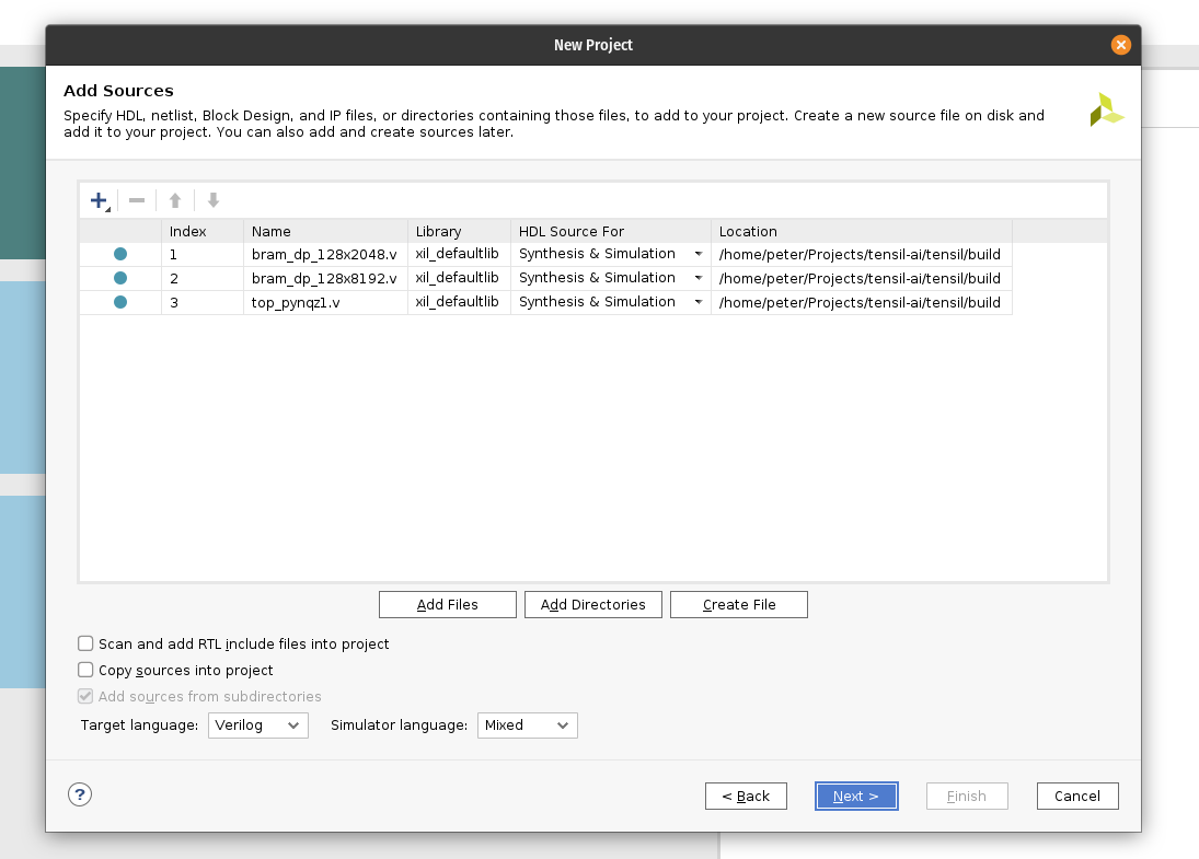
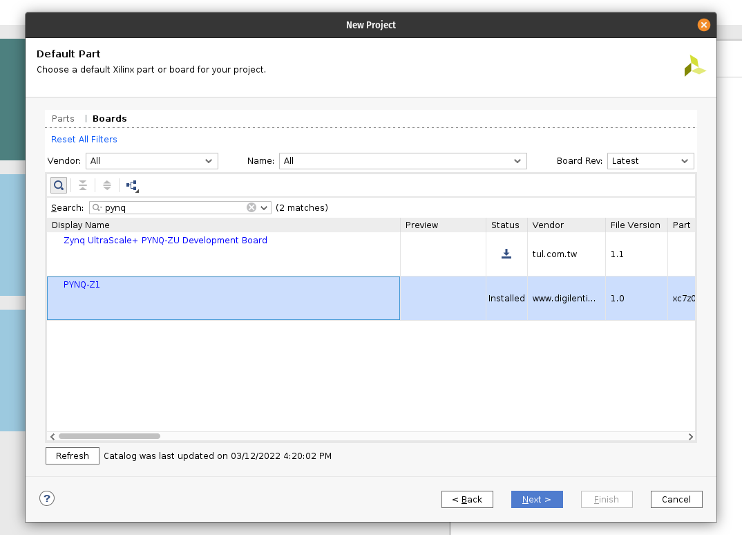
First, create a new RTL project named tensil-pynqz1 and add Verilog files generated by the Tensil RTL tool.
Choose boards and search for PYNQ. Select PYNQ-Z1 with file version 1.0.
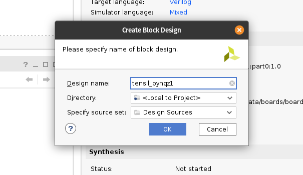
Under IP INTEGRATOR, click Create Block Design.
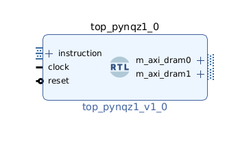
Drag top_pynqz1 from the Sources tab onto the block design diagram. You should see the Tensil RTL block with its interfaces.
Next, click the plus + button in the Block Diagram toolbar (upper left) and select “ZYNQ7 Processing System” (you may need to use the search box). Do the same for “Processor System Reset”. The Zynq block represents the “hard” part of the Xilinx platform, which includes ARM processors, DDR interfaces, and much more. The Processor System Reset is a utility box that provides the design with correctly synchronized reset signals.
Click “Run Block Automation” and “Run Connection Automation”. Check “All Automation”.
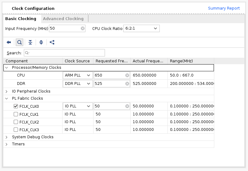
Double-click ZYNQ7 Processing System. First, go to Clock Configuration and ensure PL Fabric Clocks have FCLK_CLK0 checked and set to 50MHz.
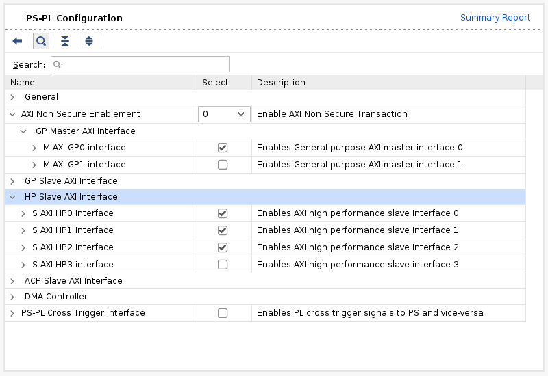
Then, go to PS-PL Configuration. Check S AXI HP0 FPD, S AXI HP1 FPD, and S AXI HP2 FPD. These changes will configure all the necessary interfaces between Processing System (PS) and Programmable Logic (PL) necessary for our design.
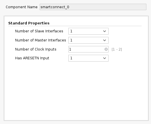
Again, click the plus + button in the Block Diagram toolbar and select “AXI SmartConnect”. We’ll need 4 instances of SmartConnect. First 3 instances (smartconnect_0 to smartconnect_2) are necessary to convert AXI version 4 interfaces of the TCU and the instruction DMA block to AXI version 3 on the PS. The smartconnect_3 is necessary to expose DMA control registers to the Zynq CPU, which will enable software to control the DMA transactions. Double-click each one and set “Number of Slave and Master Interfaces” to 1.
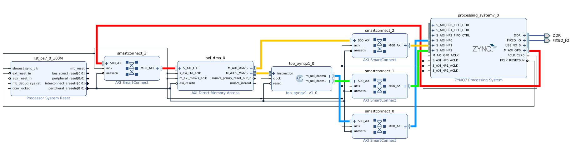
Now, connect m_axi_dram0 and m_axi_dram1 ports on Tensil block to S00_AXI on smartconnect_0 and smartconnect_1 correspondigly. Then connect SmartConnect M00_AXI ports to S_AXI_HP0 and S_AXI_HP2 on Zynq block correspondingly. The TCU has two DRAM banks to enable their parallel operation by utilizing PS ports with dedicated connectivity to the memory.
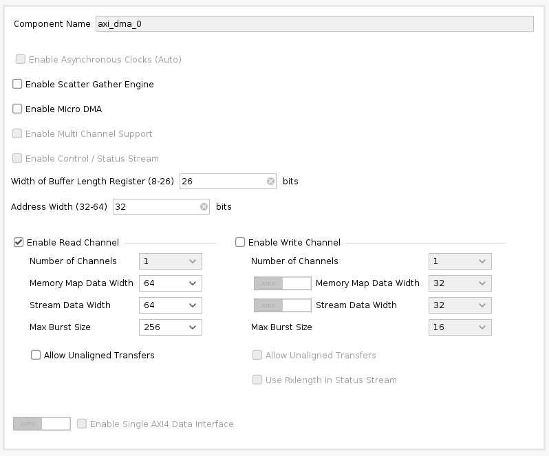
Next, click the plus + button in the Block Diagram toolbar and select “AXI Direct Memory Access” (DMA). The DMA block is used to organize the feeding of the Tensil program to the TCU without keeping the PS ARM processor busy.
Double-click it. Disable “Scatter Gather Engine” and “Write Channel”. Change “Width of Buffer Length Register” to be 26 bits. Select “Memory Map Data Width” and “Stream Data Width” to be 64 bits. Change “Max Burst Size” to 256.
Connect the instruction port on the Tensil top block to the M_AXIS_MM2S on the AXI DMA block. Then, connect M_AXI_MM2S on the AXI DMA block to S00_AXI on smartconnect_2 and, finally, connect smartconnect_2 M00_AXI port to S_AXI_HP1 on Zynq.
Connect M00_AXI on smartconnect_3 to S_AXI_LITE on the AXI DMA block. Connect S00_AXI on the AXI SmartConnect to M_AXI_GP0 on the Zynq block.
Finally, click “Run Connection Automation” and check “All Automation”. By doing this, we connect all the clocks and resets. Click the “Regenerate Layout” button in the Block Diagram toolbar to make the diagram look nice.
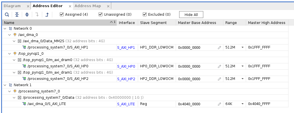
Next, switch to the “Address Editor” tab. Click the “Assign All” button in the toolbar. By doing this, we assign address spaces to various AXI interfaces. For example, the instruction DMA (axi_dma_0) and Tensil (m_axi_dram0 and m_axi_dram1) gain access to the entire address space on the PYNQ Z1 board. The PS gains access to the control registers for the instruction DMA.
Back in the Block Diagram tab, click the “Validate Design” (or F6) button. You should see the message informing you of successful validation! You can now close the Block Design by clicking x in the right upper corner.
The final step is to create the HDL wrapper for our design, which will tie everything together and enable synthesis and implementation. Right-click the tensil_pynqz1 item in the Sources tab and choose “Create HDL Wrapper”. Keep “Let Vivado manage wrapper and auto-update” selected. Wait for the Sources tree to be fully updated and right-click on tensil_pynqz1_wrapper. Choose Set as Top.
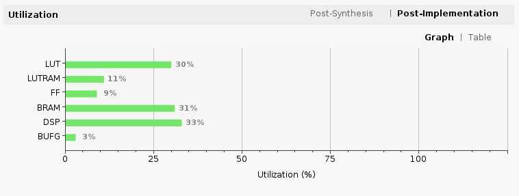
Now it’s time to let Vivado perform synthesis and implementation and write the resulting bitstream. In the Flow Navigator sidebar, click on “Generate Bitstream” and hit OK. Vivado will start synthesizing our Tensil design – this may take around 15 minutes. When done, you can observe some vital stats in the Project Summary. First, look at utilization, which shows what percentage of each FPGA resource our design is using. Note how we kept BRAM and DSP utilization reasonably low.
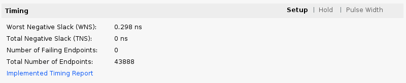
The second is timing, which tells us about how long it takes for signals to propagate in our programmable logic (PL). The “Worst Negative Slack” being a positive number is good news – our design meets propagation constraints for all nets at the specified clock speed!
5. Compile ML model for TCU
The second branch of the Tensil toolchain flow is to compile the ML model to a Tensil binary consisting of TCU instructions, which are executed by the TCU hardware directly. For this tutorial, we will use ResNet20 trained on the CIFAR dataset. The model is included in the Tensil docker image at /demo/models/resnet20v2_cifar.onnx. From within the Tensil docker container, run the following command.
tensil compile -a /demo/arch/pynqz1.tarch -m /demo/models/resnet20v2_cifar.onnx -o "Identity:0" -s true
We’re using the ONNX version of the model, but the Tensil compiler also supports TensorFlow, which you can try by compiling the same model in TensorFlow frozen graph form at /demo/models/resnet20v2_cifar.pb.
tensil compile -a /demo/arch/pynqz1.tarch -m /demo/models/resnet20v2_cifar.pb -o "Identity" -s true
The resulting compiled files are listed in the ARTIFACTS table. The manifest (tmodel) is a plain text JSON description of the compiled model. The Tensil program (tprog) and weights data (tdata) are both binaries to be used by the TCU during execution. The Tensil compiler also prints a COMPILER SUMMARY table with interesting stats for both the TCU architecture and the model.
------------------------------------------------------------------------------------------
COMPILER SUMMARY
------------------------------------------------------------------------------------------
Model:                                           resnet20v2_cifar_onnx_pynqz1
Data type:                                       FP16BP8
Array size:                                      8
Consts memory size (vectors/scalars/bits):       1,048,576                    8,388,608 20
Vars memory size (vectors/scalars/bits):         1,048,576                    8,388,608 20
Local memory size (vectors/scalars/bits):        8,192                        65,536    13
Accumulator memory size (vectors/scalars/bits):  2,048                        16,384    11
Stride #0 size (bits):                           3
Stride #1 size (bits):                           3
Operand #0 size (bits):                          16
Operand #1 size (bits):                          24
Operand #2 size (bits):                          16
Instruction size (bytes):                        8
Consts memory maximum usage (vectors/scalars):   71,341                       570,728
Vars memory maximum usage (vectors/scalars):     26,624                       212,992
Consts memory aggregate usage (vectors/scalars): 71,341                       570,728
Vars memory aggregate usage (vectors/scalars):   91,170                       729,360
Number of layers:                                23
Total number of instructions:                    258,037
Compilation time (seconds):                      25.487
True consts scalar size:                         568,466
Consts utilization (%):                          97.545
True MACs (M):                                   61.476
MAC efficiency (%):                              0.000
------------------------------------------------------------------------------------------
6. Execute using PYNQ
Now it’s time to put everything together on our development board. For this, we first need to set up the PYNQ environment. This process starts with downloading the SD card image for our development board. There’s the detailed instruction for setting board connectivity on the PYNQ documentation website. You should be able to open Jupyter notebooks and run some examples.
Now that PYNQ is up and running, the next step is to scp the Tensil driver for PYNQ. Start by cloning the Tensil GitHub repository to your work station and then copy drivers/tcu_pynq to /home/xilinx/tcu_pynq onto your board.
git clone [email protected]:tensil-ai/tensil.git
scp -r tensil/drivers/tcu_pynq [email protected]:
We also need to scp the bitstream and compiler artifacts.
Next we’ll copy over the bitstream, which contains the FPGA configuration resulting from Vivado synthesis and implementation. PYNQ also needs a hardware handoff file that describes FPGA components accessible to the host, such as DMA. Place both files in /home/xilinx on the development board. Assuming you are in the Vivado project directory, run the following commands to copy files over.
scp tensil-pynqz1.runs/impl_1/tensil_pynqz1_wrapper.bit [email protected]:tensil_pynqz1.bit
scp tensil-pynqz1.gen/sources_1/bd/tensil_pynqz1/hw_handoff/tensil_pynqz1.hwh [email protected]:
Note that we renamed bitstream to match the hardware handoff file name.
Now, copy the .tmodel, .tprog and .tdata artifacts produced by the compiler to /home/xilinx on the board.
scp resnet20v2_cifar_onnx_pynqz1.t* [email protected]:
The last thing needed to run our ResNet model is the CIFAR dataset. You can get it from Kaggle or run the commands below (since we only need the test batch, we remove the training batches to reduce the file size). Put these files in /home/xilinx/cifar-10-batches-py/ on your development board.
wget http://www.cs.toronto.edu/~kriz/cifar-10-python.tar.gz
tar xfvz cifar-10-python.tar.gz
rm cifar-10-batches-py/data_batch_*
scp -r cifar-10-batches-py [email protected]:
We are finally ready to fire up the PYNQ Jupyter notebook and run the ResNet model on TCU.
Jupyter notebook
First, we import the Tensil PYNQ driver and other required utilities.
import sys
sys.path.append('/home/xilinx')

# Needed to run inference on TCU
import time
import numpy as np
import pynq
from pynq import Overlay
from tcu_pynq.driver import Driver
from tcu_pynq.architecture import pynqz1

# Needed for unpacking and displaying image data
%matplotlib inline
import matplotlib.pyplot as plt
import pickle
Now, initialize the PYNQ overlay from the bitstream and instantiate the Tensil driver using the TCU architecture and the overlay’s DMA configuration. Note that we are passing axi_dma_0 object from the overlay – the name matches the DMA block in the Vivado design.
overlay = Overlay('/home/xilinx/tensil_pynqz1.bit')
tcu = Driver(pynqz1, overlay.axi_dma_0)
The Tensil PYNQ driver includes the PYNQ Z1 architecture definition. Here it is in an excerpt from architecture.py: you can see that it matches the architecture we used previously.
pynqz1 = Architecture(
    data_type=DataType.FP16BP8,
    array_size=8,
    dram0_depth=1048576,
    dram1_depth=1048576,
    local_depth=8192,
    accumulator_depth=2048,
    simd_registers_depth=1,
    stride0_depth=8,
    stride1_depth=8,
)
Next, let’s load CIFAR images from the test_batch.
def unpickle(file):
    with open(file, 'rb') as fo:
        d = pickle.load(fo, encoding='bytes')
    return d

cifar = unpickle('/home/xilinx/cifar-10-batches-py/test_batch')
data = cifar[b'data']
labels = cifar[b'labels']

data = data[10:20]
labels = labels[10:20]

data_norm = data.astype('float32') / 255
data_mean = np.mean(data_norm, axis=0)
data_norm -= data_mean

cifar_meta = unpickle('/home/xilinx/cifar-10-batches-py/batches.meta')
label_names = [b.decode() for b in cifar_meta[b'label_names']]

def show_img(data, n):
    plt.imshow(np.transpose(data[n].reshape((3, 32, 32)), axes=[1, 2, 0]))

def get_img(data, n):
    img = np.transpose(data_norm[n].reshape((3, 32, 32)), axes=[1, 2, 0])
    img = np.pad(img, [(0, 0), (0, 0), (0, tcu.arch.array_size - 3)], 'constant', constant_values=0)
    return img.reshape((-1, tcu.arch.array_size))

def get_label(labels, label_names, n):
    label_idx = labels[n]
    name = label_names[label_idx]
    return (label_idx, name)
To test, extract one of the images.
n = 7
img = get_img(data, n)
label_idx, label = get_label(labels, label_names, n)
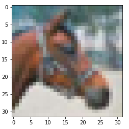
show_img(data, n)
You should see the image.
Next, load the tmodel manifest for the model into the driver. The manifest tells the driver where to find the other two binary files (program and weights data).
tcu.load_model('/home/xilinx/resnet20v2_cifar_onnx_pynqz1.tmodel')
Finally, run the model and print the results! The call to tcu.run(inputs) is where the magic happens. We’ll convert the ResNet classification result vector into CIFAR labels. Note that if you are using the ONNX model, the input and output are named x:0 and Identity:0 respectively. For the TensorFlow model they are named x and Identity.
inputs = {'x:0': img}

start = time.time()
outputs = tcu.run(inputs)
end = time.time()
print("Ran inference in {:.4}s".format(end - start))
print()

classes = outputs['Identity:0'][:10]
result_idx = np.argmax(classes)
result = label_names[result_idx]
print("Output activations:")
print(classes)
print()
print("Result: {} (idx = {})".format(result, result_idx))
print("Actual: {} (idx = {})".format(label, label_idx))
Here is the expected result:
Ran inference in 0.1513s

Output activations:
[-19.49609375 -12.37890625  -8.01953125  -6.01953125  -6.609375
  -4.921875    -7.71875      2.0859375   -9.640625    -7.85546875]

Result: horse (idx = 7)
Actual: horse (idx = 7)
Congratulations! You ran a machine learning model a custom ML accelerator that you built on your own work station! Just imagine the things you could do with it…
Wrap-up
In this tutorial we used Tensil to show how to run machine learning (ML) models on FPGA. We went through a number of steps to get here, including installing Tensil, choosing an architecture, generating an RTL design, synthesizing the desing, compiling the ML model and finally executing the model using PYNQ.
If you made it all the way through, big congrats! You’re ready to take things to the next level by trying out your own model and architecture. Join us on Discord to say hello and ask questions, or send an email to [email protected].